Meep Reference
From AbInitio
| Revision as of 00:48, 11 September 2009 (edit) Stevenj (Talk | contribs) (→source - omega vs. f clarifications) ← Previous diff |
Current revision (06:07, 25 August 2016) (edit) Ardavan (Talk | contribs) (→pml) |
||
| Line 19: | Line 19: | ||
| ; <code>pml-layers</code> [list of <code>pml</code> class] | ; <code>pml-layers</code> [list of <code>pml</code> class] | ||
| : Specifies the absorbing [[perfectly matched layers|PML]] boundary layers to use; defaults to none. | : Specifies the absorbing [[perfectly matched layers|PML]] boundary layers to use; defaults to none. | ||
| - | ; <code>default-material</code> [<code>material-type</code> class] | ||
| - | : Holds the default material that is used for points not in any object of the geometry list. Defaults to <code>air</code> (ε of 1). | ||
| ; <code>geometry-lattice</code> [<code>lattice</code> class] | ; <code>geometry-lattice</code> [<code>lattice</code> class] | ||
| : Specifies the size of the unit cell (which is centered on the origin of the coordinate system). Any sizes of <code>no-size</code> imply (effectively) a reduced-dimensionality calculation (but a 2d <math>xy</math> calculation is especially optimized); see <code>dimensions</code> below. Defaults to a cubic cell of unit size. | : Specifies the size of the unit cell (which is centered on the origin of the coordinate system). Any sizes of <code>no-size</code> imply (effectively) a reduced-dimensionality calculation (but a 2d <math>xy</math> calculation is especially optimized); see <code>dimensions</code> below. Defaults to a cubic cell of unit size. | ||
| + | ; <code>default-material</code> [<code>material-type</code> class] | ||
| + | : Holds the default material that is used for points not in any object of the geometry list. Defaults to <code>air</code> (ε of 1). See also <code>epsilon-input-file</code> below. | ||
| + | ; <code>epsilon-input-file</code> [<code>string</code>] | ||
| + | : If this string is not <code>""</code> (the default), then it should be the name of an HDF5 file whose first/only dataset defines a scalar dielectric function (over some discrete grid); alternatively, the dataset name can be specified explicitly if the string is in the form "''filename'':''dataset''". This dielectric function is then used in place of the ε property of <code>default-material</code> (''i.e.'' where there are no <code>geometry</code> objects). The grid of the epsilon file dataset need not match Meep's computational grid; it is scaled and/or linearly interpolated as needed to map the file onto the computational cell (which warps the structure if the proportions of the grids do not match, however). '''Note:''' the file contents ''only'' override the ε property of the <code>default-material</code>, whereas other properties (μ, susceptibilities, nonlinearities, etc.) of <code>default-material</code> are still used. | ||
| ; <code>dimensions</code> [<code>integer</code>] | ; <code>dimensions</code> [<code>integer</code>] | ||
| : Explicitly specifies the dimensionality of the simulation, if the value is less than 3. If the value is 3 (the default), then the dimensions are automatically reduced to 2 if possible when <code>geometry-lattice</code> size in the <math>z</math> direction is <code>no-size</code>. If <code>dimensions</code> is the special value of <code>CYLINDRICAL</code>, then cylindrical coordinates are used and the <math>x</math> and <math>z</math> dimensions are interpreted as <math>r</math> and <math>z</math>, respectively. If <code>dimensions</code> is 1, then the cell must be along the <math>z</math> direction and only <math>E_x</math> and <math>H_y</math> field components are permitted. If <code>dimensions</code> is 2, then the cell must be in the <math>xy</math> plane. | : Explicitly specifies the dimensionality of the simulation, if the value is less than 3. If the value is 3 (the default), then the dimensions are automatically reduced to 2 if possible when <code>geometry-lattice</code> size in the <math>z</math> direction is <code>no-size</code>. If <code>dimensions</code> is the special value of <code>CYLINDRICAL</code>, then cylindrical coordinates are used and the <math>x</math> and <math>z</math> dimensions are interpreted as <math>r</math> and <math>z</math>, respectively. If <code>dimensions</code> is 1, then the cell must be along the <math>z</math> direction and only <math>E_x</math> and <math>H_y</math> field components are permitted. If <code>dimensions</code> is 2, then the cell must be in the <math>xy</math> plane. | ||
| Line 143: | Line 145: | ||
| :; <code>chi3</code> [<code>number</code>] | :; <code>chi3</code> [<code>number</code>] | ||
| :: The nonlinear (Kerr) susceptibility <math>\chi^{(3)}</math>. Default value = 0. (See e.g. [[Meep Tutorial/Third harmonic generation]].) See also [[Nonlinearity in Meep]]. | :: The nonlinear (Kerr) susceptibility <math>\chi^{(3)}</math>. Default value = 0. (See e.g. [[Meep Tutorial/Third harmonic generation]].) See also [[Nonlinearity in Meep]]. | ||
| - | :; <code>E-polarizations</code> [list of <code>polarizability</code> class] | + | :; <code>E-susceptibilities</code> [list of <code>susceptibility</code> class] |
| - | :: List of dispersive polarizabilities (see below) added to the dielectric constant ε, in order to model material dispersion; defaults to none. (See e.g. [[Meep Tutorial/Material dispersion]].) See also [[Material dispersion in Meep]]. For backwards compatibility, a synonym of <code>E-polarizations</code> is <code>polarizations</code>. | + | :: List of dispersive susceptibilities (see below) added to the dielectric constant ε, in order to model material dispersion; defaults to none. (See e.g. [[Meep Tutorial/Material dispersion]].) See also [[Material dispersion in Meep]]. For backwards compatibility, synonyms of <code>E-susceptibilities</code> are <code>E-polarizations</code> and <code>polarizations</code>. |
| - | :; <code>H-polarizations</code> [list of <code>polarizability</code> class] | + | :; <code>H-susceptibilities</code> [list of <code>susceptibility</code> class] |
| - | :: List of dispersive polarizabilities (see below) added to the permeability μ, in order to model material dispersion; defaults to none. (See e.g. [[Meep Tutorial/Material dispersion]].) See also [[Material dispersion in Meep]]. | + | :: List of dispersive susceptibilities (see below) added to the permeability μ, in order to model material dispersion; defaults to none. (See e.g. [[Meep Tutorial/Material dispersion]].) See also [[Material dispersion in Meep]]. For backwards compatibility, a synonym of <code>H-susceptibilities</code> is <code>H-polarizations</code>. |
| ; <code>perfect-metal</code> | ; <code>perfect-metal</code> | ||
| : A perfectly conducting metal; this class has no properties and you normally just use the predefined <code>metal</code> object, above. (To model imperfect conductors, use a dispersive dielectric material.) See also the [[#Predefined Variables|predefined variables]] <code>metal</code>, <code>perfect-electric-conductor</code>, and <code>perfect-magnetic-conductor</code> above. | : A perfectly conducting metal; this class has no properties and you normally just use the predefined <code>metal</code> object, above. (To model imperfect conductors, use a dispersive dielectric material.) See also the [[#Predefined Variables|predefined variables]] <code>metal</code>, <code>perfect-electric-conductor</code>, and <code>perfect-magnetic-conductor</code> above. | ||
| Line 156: | Line 158: | ||
| ::'''Important:''' If your material function returns nonlinear, dispersive (Lorentzian or conducting), or magnetic materials, you should also include a list of these materials in the <code>extra-materials</code> input variable (above) to let Meep know that it needs to support these material types in your simulation. (For dispersive materials, you need to include a material with the ''same'' γ<sub>''n''</sub> and ω<sub>''n''</sub> values, so you can only have a finite number of these, whereas σ<sub>''n''</sub> can vary continuously if you want and a matching σ<sub>''n''</sub> need not be specified in <code>extra-materials</code>. For nonlinear or conductivity materials, your <code>extra-materials</code> list need not match the actual values of σ or χ returned by your material function, which can vary continuously if you want.) | ::'''Important:''' If your material function returns nonlinear, dispersive (Lorentzian or conducting), or magnetic materials, you should also include a list of these materials in the <code>extra-materials</code> input variable (above) to let Meep know that it needs to support these material types in your simulation. (For dispersive materials, you need to include a material with the ''same'' γ<sub>''n''</sub> and ω<sub>''n''</sub> values, so you can only have a finite number of these, whereas σ<sub>''n''</sub> can vary continuously if you want and a matching σ<sub>''n''</sub> need not be specified in <code>extra-materials</code>. For nonlinear or conductivity materials, your <code>extra-materials</code> list need not match the actual values of σ or χ returned by your material function, which can vary continuously if you want.) | ||
| - | '''Complex ε and μ''': you cannot specify a frequency-independent complex ε or μ in Meep (where the imaginary part is a frequency-independent loss), but there is an alternative. That is because there are only two important physical situations. First, if you only care about the loss in a narrow bandwidth around some frequency, you can set the loss at that frequency via the conductivity (see [[Conductivity in Meep]]). Second, if you care about a broad bandwidth, then all physical materials have a frequency-dependent imaginary (and real) ε (and/or μ), and you need to specify that frequency dependence by fitting to Lorentzian resonances via the <code>polarizability</code> below. | + | '''Complex ε and μ''': you cannot specify a frequency-independent complex ε or μ in Meep (where the imaginary part is a frequency-independent loss), but there is an alternative. That is because there are only two important physical situations. First, if you only care about the loss in a narrow bandwidth around some frequency, you can set the loss at that frequency via the conductivity (see [[Conductivity in Meep]]). Second, if you care about a broad bandwidth, then all physical materials have a frequency-dependent imaginary (and real) ε (and/or μ), and you need to specify that frequency dependence by fitting to Lorentzian (and/or Drude) resonances via the <code>lorentzian-susceptibility</code> (or <code>drude-susceptibility</code>) classes below. |
| - | Dispersive dielectric materials, above, are specified via a list of objects of type <code>polarizability</code>, which is another class with four properties: | + | Dispersive dielectric (and magnetic) materials, above, are specified via a list of objects that are subclasses of type <code>susceptibility</code>. |
| - | ; <code>polarizability</code> | + | ; <code>susceptibility</code> |
| - | : Specifies a single dispersive polarizability of damped harmonic form (see [[Material dispersion in Meep]]), with the parameters: | + | : Parent class for various dispersive susceptibility terms, parameterized by an anisotropic amplitude σ (see [[Material dispersion in Meep]]): |
| - | :; <code>omega</code> [<code>number</code>] | + | :; <code>sigma</code> [<code>number</code>] |
| + | :: The scale factor σ. You can also specify an anisotropic σ tensor by using the property <code>sigma-diag</code> [<math>vector3</math>], which takes three numbers or a <math>vector3</math> to give the <math>\sigma_n</math> tensor diagonal, and <code>sigma-offdiag</code> [<math>vector3</math>] which specifies the offdiagonal elements (defaults to 0). That is, <code>(sigma-diag a b c)</code> and <code>(sigma-offdiag u v w)</code> corresponds to a σ tensor | ||
| + | ::<math>\sigma = | ||
| + | \begin{pmatrix} | ||
| + | a & u & v \\ | ||
| + | u & b & w \\ | ||
| + | v & w & c | ||
| + | \end{pmatrix}</math> | ||
| + | ; <code>lorentzian-susceptibility</code> | ||
| + | : Specifies a single dispersive susceptibility of Lorentzian (damped harmonic oscillator) form (see [[Material dispersion in Meep]]), with the parameters (in addition to σ): | ||
| + | :; <code>frequency</code> [<code>number</code>] | ||
| :: The resonance frequency <math>f_n = \omega_n / 2\pi</math>. | :: The resonance frequency <math>f_n = \omega_n / 2\pi</math>. | ||
| :; <code>gamma</code> [<code>number</code>] | :; <code>gamma</code> [<code>number</code>] | ||
| :: The resonance loss rate <math>\gamma_n / 2\pi</math>. | :: The resonance loss rate <math>\gamma_n / 2\pi</math>. | ||
| - | :; <code>sigma</code> [<code>number</code>] | + | ; <code>drude-susceptibility</code> |
| - | :: The scale factor <math>\sigma_n</math>. You can also specify an diagonal anisotropic σ tensor by using the property <code>sigma-diag</code> [<math>vector3</math>], which takes three numbers or a <math>vector3</math> to give the <math>\sigma_n</math> tensor diagonal. See also [[Material dispersion in Meep]]. | + | : Specifies a single dispersive susceptibility of Drude form (see [[Material dispersion in Meep]]), with the parameters (in addition to σ): |
| + | :; <code>frequency</code> [<code>number</code>] | ||
| + | :: The frequency scale factor <math>f_n = \omega_n / 2\pi</math> which multiplies σ (not a resonance frequency). | ||
| + | :; <code>gamma</code> [<code>number</code>] | ||
| + | :: The loss rate <math>\gamma_n / 2\pi</math>. | ||
| + | |||
| + | Meep also supports a somewhat unusual polarizable medium, a Lorentzian susceptibility with a random noise term added into the damped-oscillator equation at each point. This can be used to directly model thermal radiation in both the far field (as described in [http://journals.aps.org/prl/abstract/10.1103/PhysRevLett.93.213905 Luo et al., 2004]) and the near field (as described in [http://math.mit.edu/~stevenj/papers/RodriguezIl11.pdf Rodriguez et al., 2011]). (Note, however that it is more efficient to compute far-field thermal radiation using Kirchhoff's law of radiation, which states that emissivity equals absorptivity. Near-field thermal radiation can usually be computed more efficiently using frequency domain techniques, e.g. via our [http://homerreid.dyndns.org/scuff-EM/ SCUFF-EM] code, as described by [http://math.mit.edu/~stevenj/papers/RodriguezRe13-heat.pdf Rodriguez et al., 2013].) | ||
| + | ; <code>noisy-lorentzian-susceptibility</code> or <code>noisy-drude-susceptibility</code> | ||
| + | : Specifies a single dispersive susceptibility of Lorentzian (damped harmonic oscillator) or Drude form (see [[Material dispersion in Meep]]), with the same σ, <code>frequency</code>, and <code>gamma</code>) parameters, but with an additional Gaussian random noise term (uncorrelated in space and time, zero mean) added to the '''P''' damped-oscillator equation. | ||
| + | :; <code>noise-amp</code> [<code>number</code>] | ||
| + | :: The noise has root-mean square amplitude σ⋅<code>noise-amp</code>. | ||
| === geometric-object === | === geometric-object === | ||
| Line 256: | Line 278: | ||
| ; <code>pml</code> | ; <code>pml</code> | ||
| - | : A single PML layer specification, which sets up one or more PML layers around the boundaries according to the following four properties. | + | : A single PML layer specification, which sets up one or more PML layers around the boundaries according to the following properties. |
| :; <code>thickness</code> [<code>number</code>] | :; <code>thickness</code> [<code>number</code>] | ||
| :: The spatial thickness of the PML layer (which extends from the boundary towards the ''inside'' of the computational cell). The thinner it is, the more numerical reflections become a problem. No default value. | :: The spatial thickness of the PML layer (which extends from the boundary towards the ''inside'' of the computational cell). The thinner it is, the more numerical reflections become a problem. No default value. | ||
| Line 266: | Line 288: | ||
| :: A strength (default is <code>1.0</code>) to multiply the PML absorption coefficient by. A strength of <code>2.0</code> will ''square'' the theoretical asymptotic reflection coefficient of the PML (making it smaller), but will also increase numerical reflections. Alternatively, you can change <code>R-asymptotic</code>, below. | :: A strength (default is <code>1.0</code>) to multiply the PML absorption coefficient by. A strength of <code>2.0</code> will ''square'' the theoretical asymptotic reflection coefficient of the PML (making it smaller), but will also increase numerical reflections. Alternatively, you can change <code>R-asymptotic</code>, below. | ||
| :; <code>R-asymptotic</code> [<code>number</code>] | :; <code>R-asymptotic</code> [<code>number</code>] | ||
| - | ::The asymptotic reflection in the limit of infinite resolution or infinite PML thickness, for refections from air (an upper bound for other media with index > 1). (For a finite resolution or thickness, the reflection will be ''much larger'', due to the discretization of Maxwell's equation.) The default value is 10<sup>−15</sup>, which should be suffice for most purposes. (You want to set this to be small enough so that waves propagating within the PML are attenuated sufficiently, but making <code>R-asymptotic</code> too small will increase the numerical reflection due to discretization.) | + | ::The asymptotic reflection in the limit of infinite resolution or infinite PML thickness, for refections from air (an upper bound for other media with index > 1). (For a finite resolution or thickness, the reflection will be ''much larger'', due to the discretization of Maxwell's equation.) The default value is 10<sup>−15</sup>, which should suffice for most purposes. (You want to set this to be small enough so that waves propagating within the PML are attenuated sufficiently, but making <code>R-asymptotic</code> too small will increase the numerical reflection due to discretization.) |
| :; <code>pml-profile</code> [<code>function</code>] | :; <code>pml-profile</code> [<code>function</code>] | ||
| :: By default, Meep turns on the PML conductivity quadratically within the PML layer—one doesn't want to turn it on suddenly, because that exacerbates reflections due to the discretization. More generally, with <code>pml-profile</code> one can specify an arbitrary PML "profile" function ''f''(''u'') that determines the shape of the PML absorption profile up to an overall constant factor. ''u'' goes from 0 to 1 at the start and end of the PML, and the default is ''f''(''u'')=''u''<sup>2</sup>. In some cases where a very thick PML is required, such as in a periodic medium (where there is technically no such thing as a true PML, only a pseudo-PML), it can be advantageous to turn on the PML absorption more smoothly (see [http://www.opticsinfobase.org/abstract.cfm?URI=oe-16-15-11376 Oskooi et al., 2008]). For example, one can use a cubic profile ''f''(''u'')=''u''<sup>3</sup> by specifying <code>(pml-profile (lambda (u) (* u u u)))</code>. | :: By default, Meep turns on the PML conductivity quadratically within the PML layer—one doesn't want to turn it on suddenly, because that exacerbates reflections due to the discretization. More generally, with <code>pml-profile</code> one can specify an arbitrary PML "profile" function ''f''(''u'') that determines the shape of the PML absorption profile up to an overall constant factor. ''u'' goes from 0 to 1 at the start and end of the PML, and the default is ''f''(''u'')=''u''<sup>2</sup>. In some cases where a very thick PML is required, such as in a periodic medium (where there is technically no such thing as a true PML, only a pseudo-PML), it can be advantageous to turn on the PML absorption more smoothly (see [http://www.opticsinfobase.org/abstract.cfm?URI=oe-16-15-11376 Oskooi et al., 2008]). For example, one can use a cubic profile ''f''(''u'')=''u''<sup>3</sup> by specifying <code>(pml-profile (lambda (u) (* u u u)))</code>. | ||
| + | |||
| + | ==== absorber ==== | ||
| + | |||
| + | Instead of a <code>pml</code> layer, there is an alternative class called <code>absorber</code> which is a '''drop-in''' replacement for <code>pml</code>. For example, you can do <code>(set! pml-layers (list (make absorber (thickness 2))))</code> instead of <code>(set! pml-layers (list (make pml (thickness 2))))</code>. All the parameters are the same as for <code>pml</code>, above. You can have a mix of <code>pml</code> on some boundaries and <code>absorber</code> on others. | ||
| + | |||
| + | The <code>absorber</code> class does ''not'' implement a perfectly matched layer (PML), however (except in 1d). Instead, it is simply a scalar electric '''and''' magnetic conductivity that turns on gradually within the layer according to the <code>pml-profile</code> (defaulting to quadratic). Such a scalar conductivity gradient is only reflectionless in the limit as the layer becomes sufficiently thick. | ||
| + | |||
| + | The main reason to use <code>absorber</code> is if you have '''a case in which PML fails:''' | ||
| + | * No true PML exists for ''periodic'' media, and a scalar absorber is cheaper and is generally just as good. See [http://math.mit.edu/~stevenj/papers/papers_abstracts.html#OskooiZh08 Oskooi et al. (2008)]. | ||
| + | * PML can lead to ''divergent'' fields for certain waveguides with "backward-wave" modes; this can easily happen in metallic with surface plasmons, and a scalar absorber is your only choice. See [http://math.mit.edu/~stevenj/papers/papers_abstracts.html#LohOs09 Loh et al. (2009)]. | ||
| + | * PML can fail if you have a waveguide hitting the edge of your computational cell ''at an angle''. See [http://math.mit.edu/~stevenj/papers/papers_abstracts.html#OskooiJo11 Oskooi et. al. (2011).] | ||
| === source === | === source === | ||
| Line 274: | Line 307: | ||
| The <code>source</code> class is used to specify the current sources (via the <code>sources</code> input variable). Note that all sources in Meep are separable in time and space, i.e. of the form <math>\mathbf{J}(\mathbf{x},t) = \mathbf{A}(\mathbf{x}) \cdot f(t)</math> for some functions <math>\mathbf{A}</math> and <math>f</math>. (Non-separable sources can be simulated, however, by modifying the sources after each time step.) When real fields are being used (which is the default in many cases...see the <code>force-complex-fields?</code> input variable), only the real part of the current source is used by Meep. | The <code>source</code> class is used to specify the current sources (via the <code>sources</code> input variable). Note that all sources in Meep are separable in time and space, i.e. of the form <math>\mathbf{J}(\mathbf{x},t) = \mathbf{A}(\mathbf{x}) \cdot f(t)</math> for some functions <math>\mathbf{A}</math> and <math>f</math>. (Non-separable sources can be simulated, however, by modifying the sources after each time step.) When real fields are being used (which is the default in many cases...see the <code>force-complex-fields?</code> input variable), only the real part of the current source is used by Meep. | ||
| - | '''Important note''': These are ''current'' sources ('''J''' terms in Maxwell's equations), even though they are labelled by electric/magnetic field components. They do ''not'' specify a particular electric/magnetic field (which would be what is called a "hard" source in the FDTD literature). There is no fixed relationship between the current source and the resulting field amplitudes; it depends on the surrounding geometry, as described in the [[Meep FAQ#How does the current amplitude relate to the resulting field amplitude?|Meep FAQ]]. | + | '''Important note''': These are ''current'' sources ('''J''' terms in Maxwell's equations), even though they are labelled by electric/magnetic field components. They do ''not'' specify a particular electric/magnetic field (which would be what is called a "hard" source in the FDTD literature). There is no fixed relationship between the current source and the resulting field amplitudes; it depends on the surrounding geometry, as described in the [[Meep FAQ#How does the current amplitude relate to the resulting field amplitude?|Meep FAQ]] and in [http://arxiv.org/abs/arXiv:1301.5366 our book chapter online]. |
| ; <code>source</code> | ; <code>source</code> | ||
| Line 290: | Line 323: | ||
| :;<code>amp-func</code> [<code>function</code>] | :;<code>amp-func</code> [<code>function</code>] | ||
| ::A Scheme function of a single argument, that takes a vector3 giving a position and returns a (complex) current amplitude for that point. The position argument is ''relative'' to the <code>center</code> of the current source, so that you can move your current around without changing your function. The default is <code>'()</code> (null), meaning that a constant amplitude of 1.0 is used. Note that your amplitude function (if any) is ''multiplied'' by the <code>amplitude</code> property, so both properties can be used simultaneously. | ::A Scheme function of a single argument, that takes a vector3 giving a position and returns a (complex) current amplitude for that point. The position argument is ''relative'' to the <code>center</code> of the current source, so that you can move your current around without changing your function. The default is <code>'()</code> (null), meaning that a constant amplitude of 1.0 is used. Note that your amplitude function (if any) is ''multiplied'' by the <code>amplitude</code> property, so both properties can be used simultaneously. | ||
| + | |||
| + | As described in section 4.2 of [http://arxiv.org/abs/arXiv:1301.5366 our book chapter online], it is also possible to supply a source that is designed to couple exclusively into a single waveguide mode (or other mode of some cross section or periodic region) at a single frequency, and which couples primarily into that mode as long as the bandwidth is not too broad. This is possible if you have [[MPB]] (version 1.5 or later) installed: Meep will call MPB to compute the field profile of the desired mode, and uses the field profile to produce an equivalent current source. (Note: this feature does ''not'' work in cylindrical coordinates.) To do this, instead of a <code>source</code> you should use an <code>eigenmode-source</code>: | ||
| + | |||
| + | ; <code>eigenmode-source</code> | ||
| + | : This is a subclass of <code>source</code> and has '''all of the properties''' of <code>source</code> above. However, you normally do not specify a <code>component</code>. Instead of <code>component</code>, the current source components and amplitude profile are computed by calling MPB to compute the modes of the dielectric profile in the region given by the <code>size</code> and <code>center</code> of the source, with the modes computed as if the ''source region were repeated periodically in all directions''. (If an <code>amplitude</code> and/or <code>amp-func</code> are supplied, they are ''multiplied'' by this current profile.) The desired eigenmode and other features are specified by the following properties: | ||
| + | :; <code>eig-band</code> [<code>integer</code>] | ||
| + | :: The index ''n'' (1,2,3,...) of the desired band ω<sub>''n''</sub>('''k''') to compute in MPB (1 denotes the lowest-frequency band at a given '''k''' point, and so on). | ||
| + | :; <code>direction</code> [<code>X</code>, <code>Y</code>, or <code>Z</code>; default <code>AUTOMATIC</code>], <code>eig-match-freq?</code> [<code>boolean</code>; default <code>true</code>], <code>eig-kpoint</code> [<code>vector3</code>] | ||
| + | :: By default (if <code>eig-match-freq?</code> is <code>true</code>), Meep tries to find a mode with the same frequency ω<sub>''n''</sub>('''k''') as the <code>src</code> property (above), by scanning '''k''' vectors in the given <code>direction</code> (using MPB's [[MPB User Reference#The inverse problem: k as a function of frequency|find-k]] functionality; alternatively, if <code>eig-kpoint</code> is supplied, it is used as an initial guess and direction for '''k''' ). By default, <code>direction</code> is the direction normal to the source region, assuming <code>size</code> is ''d''–1 dimensional in a ''d''-dimensional simulation (e.g. a plane in 3d). Alternatively (if <code>eig-match-freq?</code> is <code>false</code>), you can specify a particular '''k''' vector of the desired mode with <code>eig-kpoint</code> (in Meep units of 2π/''a''). | ||
| + | :; <code>eig-parity</code> [<code>NO-PARITY</code> (= default), <code>EVEN-Z</code> (= <code>TE</code>), <code>ODD-Z</code> (= <code>TM</code>), <code>EVEN-Y</code>, <code>ODD-Y</code>] | ||
| + | :: The [[MPB User Reference#Parity|parity]] (= polarization in 2d) of the mode to calculate, assuming the structure has ''z'' and/or ''y'' mirror symmetry ''in the source region''. If the structure has both ''y'' and ''z'' mirror symmetry, you can combine more than one of these, e.g. <code>EVEN-Z + ODD-Y</code>. The default is <code>NO-PARITY</code>, in which case MPB computes all of the bands (which will still be even or odd if the structure has mirror symmetry, of course). This is especially useful in 2d simulations to restrict yourself to a desired polarization. | ||
| + | :; <code>eig-resolution</code> [<code>integer</code>, defaults to same as Meep resolution] | ||
| + | :: The spatial resolution to use in MPB for the eigenmode calculations. This defaults to the same resolution as Meep, but you can use a higher resolution (in which case the structure is linearly interpolated from the Meep pixels). | ||
| + | :; <code>eig-tolerance</code> [<code>number</code>, defaults to 10<sup>–7</sup>] | ||
| + | :: The [[MPB User Reference#Input Variables|tolerance]] to use in the MPB eigensolver. (MPB terminates when the eigenvalues stop changing to less than this fractional tolerance.) | ||
| + | :; <code>component</code> [as above, but defaults to <code>ALL-COMPONENTS</code>] | ||
| + | :: Once the MPB modes are computed, equivalent electric and magnetic sources are created within Meep. By default, these sources include magnetic and electric currents in ''all'' transverse directions within the source region, corresponding to the mode fields as described in our book chapter. If you specify a <code>component</code> property, however, you can include only one component of these currents if you wish. Most people won't need this feature. | ||
| + | :; <code>eig-lattice-size</code> [<code>vector3</code>], <code>eig-lattice-center</code> [<code>vector3</code>] | ||
| + | :: Normally, the MPB computational unit cell is the same as the source volume (given by the <code>size</code> and <code>center</code> parameters). However, occasionally you want the unit cell to be larger than the source volume. For example, to create an eigenmode source in a periodic medium (photonic crystal), you need to pass MPB the entire unit cell of the periodic medium, but once the mode is computed then the actual current sources need only lie on a cross section of that medium. To accomplish this, you can specify the optional <code>eig-lattice-size</code> and <code>eig-lattice-center</code>, which define a volume (which must enclose <code>size</code> and <code>center</code>) that is used for the unit cell in MPB (with the dielectric function ε taken from the corresponding region in the Meep simulation). | ||
| + | |||
| + | Note that MPB only supports dispersionless non-magnetic materials (but it does support anisotropic ε). Any nonlinearities, magnetic responses µ, conductivities σ, or dispersive polarizations in your materials will be ''ignored'' when computing the eigenmode source. PML will also be ignored. | ||
| The <code>src-time</code> object, which specifies the time dependence of the source, can be one of the following three classes. | The <code>src-time</code> object, which specifies the time dependence of the source, can be one of the following three classes. | ||
| Line 306: | Line 360: | ||
| ::How many <code>width</code>s the current decays for before we cut it off and set it to zero; the default is <code>3.0</code>. A larger value of <code>cutoff</code> will reduce the amount of high-frequency components that are introduced by the start/stop of the source, but will of course lead to longer simulation times. | ::How many <code>width</code>s the current decays for before we cut it off and set it to zero; the default is <code>3.0</code>. A larger value of <code>cutoff</code> will reduce the amount of high-frequency components that are introduced by the start/stop of the source, but will of course lead to longer simulation times. | ||
| ; <code>gaussian-src</code> | ; <code>gaussian-src</code> | ||
| - | : A Gaussian-pulse source roughly proportional to <math>\exp(-i\omega t - (t-t_0)^2/2w^2)</math>, It has the properties: | + | : A Gaussian-pulse source roughly proportional to <math>\exp(-i\omega t - (t-t_0)^2/2w^2)</math>. Technically, the "Gaussian" sources in Meep are the (discrete-time) derivative of a Gaussian, i.e. they are <math>(-i\omega)^{-1} \frac{\partial}{\partial t} \exp(-i\omega t - (t-t_0)^2/2w^2)</math>, but the difference between this and a true Gaussian is usually irrelevant. It has the properties: |
| :;<code>frequency</code> [<code>number</code>] | :;<code>frequency</code> [<code>number</code>] | ||
| ::The center frequency ''f'' in units of c/distance (or ω in units of 2πc/distance) (see [[Meep Introduction#Units in Meep|Units in Meep]]). No default value. You can instead specify <code>(wavelength x)</code> or <code>(period x)</code>, which are both a synonym for <code>(frequency (/ 1 x))</code>; i.e. 1/ω in these units is the vacuum wavelength or the temporal period. | ::The center frequency ''f'' in units of c/distance (or ω in units of 2πc/distance) (see [[Meep Introduction#Units in Meep|Units in Meep]]). No default value. You can instead specify <code>(wavelength x)</code> or <code>(period x)</code>, which are both a synonym for <code>(frequency (/ 1 x))</code>; i.e. 1/ω in these units is the vacuum wavelength or the temporal period. | ||
| Line 312: | Line 366: | ||
| ::The width <math>w</math> used in the Gaussian. No default value. You can instead specify <code>(fwidth x)</code>, which is a synonym for <code>(width (/ 1 x))</code> (i.e. the frequency width is proportional to the inverse of the temporal width). | ::The width <math>w</math> used in the Gaussian. No default value. You can instead specify <code>(fwidth x)</code>, which is a synonym for <code>(width (/ 1 x))</code> (i.e. the frequency width is proportional to the inverse of the temporal width). | ||
| :;<code>start-time</code> [<code>number</code>] | :;<code>start-time</code> [<code>number</code>] | ||
| - | ::The starting time for the source; default is <code>0</code> (turn on at <math>t=0</math>). | + | ::The starting time for the source; default is <code>0</code> (turn on at <math>t=0</math>). (Not the time of the peak! See below.) |
| :;<code>cutoff</code> [<code>number</code>] | :;<code>cutoff</code> [<code>number</code>] | ||
| - | ::How many <code>width</code>s the current decays for before we cut it off and set it to zero—this applies for both turn-on and turn-off of the pulse. The default is <code>5.0</code>. A larger value of <code>cutoff</code> will reduce the amount of high-frequency components that are introduced by the start/stop of the source, but will of course lead to longer simulation times. | + | ::How many <code>width</code>s the current decays for before we cut it off and set it to zero—this applies for both turn-on and turn-off of the pulse. The default is <code>5.0</code>. A larger value of <code>cutoff</code> will reduce the amount of high-frequency components that are introduced by the start/stop of the source, but will of course lead to longer simulation times. The peak of the gaussian is reached at the time ''t''<sub>0</sub>= <code>start-time</code> + <code>cutoff</code>*<code>width</code>. |
| ; <code>custom-src</code> | ; <code>custom-src</code> | ||
| : A user-specified source function <math>f(t)</math>. You can also specify start/end times (at which point your current is set to zero whether or not your function is actually zero). These are optional, but you ''must specify'' an <code>end-time</code> explicitly if you want functions like <code>run-sources</code> to work, since they need to know when your source turns off. | : A user-specified source function <math>f(t)</math>. You can also specify start/end times (at which point your current is set to zero whether or not your function is actually zero). These are optional, but you ''must specify'' an <code>end-time</code> explicitly if you want functions like <code>run-sources</code> to work, since they need to know when your source turns off. | ||
| Line 378: | Line 432: | ||
| ;<code>(use-output-directory [dirname])</code> | ;<code>(use-output-directory [dirname])</code> | ||
| - | :Put output in a subdirectory, which is created if necessary. If the optional argument dirname is specified, that that is the name of the directory. Otherwise, the directory name is the current ctl file name with <code>".ctl"</code> replaced by <code>"-out"</code>: e.g. <code>tst.ctl</code> implies a directory of <code>"tst-out"</code>. | + | :Put output in a subdirectory, which is created if necessary. If the optional argument dirname is specified, that is the name of the directory. Otherwise, the directory name is the current ctl file name with <code>".ctl"</code> replaced by <code>"-out"</code>: e.g. <code>tst.ctl</code> implies a directory of <code>"tst-out"</code>. |
| === Misc. === | === Misc. === | ||
| Line 484: | Line 538: | ||
| ;<code>(scale-flux-fields s flux)</code> | ;<code>(scale-flux-fields s flux)</code> | ||
| :Scale the Fourier-transformed fields in <code>flux</code> by the complex number <code>s</code>. e.g. <code>load-minus-flux</code> is equivalent to <code>load-flux</code> followed by <code>scale-flux-fields</code> with <code>s=-1</code>. | :Scale the Fourier-transformed fields in <code>flux</code> by the complex number <code>s</code>. e.g. <code>load-minus-flux</code> is equivalent to <code>load-flux</code> followed by <code>scale-flux-fields</code> with <code>s=-1</code>. | ||
| + | |||
| + | === Force spectra === | ||
| + | |||
| + | Very similar to flux spectra, you can also compute '''force spectra''': forces on an object as a function of frequency, computed by Fourier transforming the fields and integrating the vacuum [[w:Maxwell stress tensor|Maxwell stress tensor]] | ||
| + | |||
| + | :<math>\sigma_{ij} = E_i^*E_j + H_i^*H_j - \frac{1}{2} \delta_{ij} \left( |\mathbf{E}|^2 + |\mathbf{H}|^2 \right)</math> | ||
| + | |||
| + | over a surface ''S'' via <math>\mathbf{F} = \int_S \sigma d\mathbf{A}</math>. We recommend that you normally '''only evaluate the stress tensor over a surface lying in vacuum''', as the interpretation and definition of the stress tensor in arbitrary media is often problematic (the subject of extensive and controversial literature). (It is fine if the surface ''encloses'' an object made of arbitrary materials, as long as the surface itself is in vacuum.) | ||
| + | |||
| + | See also the [[Meep Tutorial/Optical forces|optical forces Meep tutorial]]. | ||
| + | |||
| + | Most commonly, you will want to '''normalize''' the force spectrum in some way, just as for flux spectra. Most simply, you could divide two different force spectra to compute the ratio of forces on two objects. Often, you will divide a force spectrum by a flux spectrum, to divide the force ''F'' by the incident power ''P'' on an object, in order to compute the useful dimensionless ratio ''Fc''/''P'' (where ''c''=1 in Meep units). For example, it is a simple exercise to show that the force ''F'' on a perfectly reflecting mirror with normal-incident power ''P'' satisfies ''Fc''/''P''=2, and for a perfectly absorbing (black) surface ''Fc''/''P''=1. | ||
| + | |||
| + | The usage is similar to the flux spectra: you define a set of <code>force-region</code> objects telling Meep where it should compute the Fourier-transformed fields and stress tensors, and call <code>add-force</code> to add these regions to the current simulation over a specified frequency bandwidth, and then use <code>display-forces</code> to display the force spectra at the end. There are also <code>save-force</code>, <code>load-force</code>, and <code>load-minus-force</code> functions that you can use to subtract the fields from two simulation, e.g. in order to compute just the force from scattered fields, similar to the flux spectra. These types and functions are defined as follows: | ||
| + | |||
| + | ;<code>force-region</code> | ||
| + | :A region (volume, plane, line, or point) in which to compute the integral of the stress tensor of the Fourier-transformed fields. Its properties are: | ||
| + | :;<code>center</code> [<code>vector3</code>] | ||
| + | ::The center of the force region (no default). | ||
| + | :;<code>size</code> [<code>vector3</code>] | ||
| + | ::The size of the force region along each of the coordinate axes; default is (0,0,0) (a single point). | ||
| + | :;<code>direction</code> [<code>direction</code> constant] | ||
| + | ::The direction of the force that you wish to compute (e.g. <code>X</code>, <code>Y</code>, etcetera). Unlike <code>flux-region</code>, you must specify this explicitly, because there is not generally any relationship between the direction of the force and the orientation of the force region. | ||
| + | :;<code>weight</code> [<code>cnumber</code>] | ||
| + | ::A weight factor to multiply the force by when it is computed; default is <code>1.0</code>. | ||
| + | |||
| + | In most circumstances, you should define a set of <code>force-region</code>s whose union is a closed surface (lying in vacuum and enclosing the object that is experiencing the force). | ||
| + | |||
| + | ;<code>(add-force fcen df nfreq force-regions...)</code> | ||
| + | :Add a bunch of <code>force-region</code>s to the current simulation (initializing the fields if they have not yet been initialized), telling Meep to accumulate the appropriate field Fourier transforms for <code>nfreq</code> equally spaced frequencies covering the frequency range <code>fcen-df/2</code> to <code>fcen+df/2</code>. Return a ''force object'', which you can pass to the functions below to get the force spectrum, etcetera. | ||
| + | |||
| + | As for flux regions, you normally use <code>add-force</code> via statements like: | ||
| + | |||
| + | (define Fx (add-force ...)) | ||
| + | |||
| + | to store the flux object in a variable. <code>add-force</code> initializes the fields if necessary, just like calling <code>run</code>, so you should only call it ''after'' setting up your <code>geometry</code>, <code>sources</code>, <code>pml-layers</code>, etcetera. You can create as many force objects as you want, e.g. to look at forces on different objects, in different directions, or in different frequency ranges. Note, however, that Meep has to store (and update at every time step) a number of Fourier components equal to the number of grid points intersecting the force region, multiplied by the number of electric and magnetic field components required to get the stress vector, multiplied by <code>nfreq</code>, so this can get quite expensive (in both memory and time) if you want a lot of frequency points over large regions of space. | ||
| + | |||
| + | Once you have called <code>add-force</code>, the Fourier transforms of the fields are accumulated automatically during time-stepping by the <code>run</code> functions. At any time, you can ask for Meep to print out the current force spectrum via: | ||
| + | |||
| + | ;<code>(display-forces forces...)</code> | ||
| + | :Given a number of force objects, this displays a comma-separated table of frequencies and force spectra, prefixed by "force1:" or similar (where the number is incremented after each run). All of the forces should be for the same <code>fcen</code>/<code>df</code>/<code>nfreq</code>. The first column are the frequencies, and subsequent columns are the force spectra. | ||
| + | |||
| + | You might have to do something lower-level if you have multiple force regions corresponding to ''different'' frequency ranges, or have other special needs. <code>(display-forces f1 f2 f3)</code> is actually equivalent to <code>(display-csv "force" (get-force-freqs f1) (get-forces f1) (get-forces f2) (get-forces f3)</code>, where <code>display-csv</code> takes a bunch of lists of numbers and prints them as a comma-separated table, and we are calling two lower-level functions: | ||
| + | |||
| + | ;<code>(get-force-freqs flux)</code> | ||
| + | :Given a force object, returns a list of the frequencies that it is computing the spectrum for. | ||
| + | ;<code>(get-forces flux)</code> | ||
| + | :Given a force object, returns a list of the current force spectrum that it has accumulated. | ||
| + | |||
| + | As described in the [[Meep tutorial]], to compute the force from scattered fields often want to save the Fourier-transformed fields from a "normalization" run and then load them into another run to be subtracted. This can be done via: | ||
| + | |||
| + | ;<code>(save-force filename force)</code> | ||
| + | :Save the Fourier-transformed fields corresponding to the given force object in an HDF5 file of the given name (without the ".h5" suffix) (the current filename-prefix is prepended automatically). | ||
| + | ;<code>(load-force filename force)</code> | ||
| + | :Load the Fourier-transformed fields into the given force object (replacing any values currently there) from an HDF5 file of the given name (without the ".h5" suffix) (the current filename-prefix is prepended automatically). You must load from a file that was saved by <code>save-force</code> in a simulation of ''the same dimensions'' (for both the computational cell and the force regions) with the ''same number of processors''. | ||
| + | ;<code>(load-minus-force filename force)</code> | ||
| + | :As <code>load-force</code>, but negates the Fourier-transformed fields after they are loaded. This means that they will be ''subtracted'' from any future field Fourier transforms that are accumulated. | ||
| + | |||
| + | === LDOS spectra === | ||
| + | |||
| + | Meep can also calculate the LDOS (local density of states) spectrum, as described in the [[Meep Tutorial/Local density of states|Meep LDOS tutorial]]. To do this, you simply pass the following step function to your <code>run</code> command: | ||
| + | |||
| + | ;<code>(dft-ldos fcen df nfreq)</code> | ||
| + | :Compute the power spectrum of the sources (usually a single point dipole source), normalized to correspond to the LDOS, in a frequency bandwith <code>df</code> centered at <code>fcen</code>, at <code>nfreq</code> frequency points. | ||
| + | |||
| + | The resulting spectrum is outputted as comma-delimited text, prefixed by <code>ldos:,</code>, and is also stored in the <code>dft-ldos-data</code> global variable (after the <code>run</code> is complete). | ||
| + | |||
| + | Analytically, the per-polarization LDOS is exactly proportional to the power radiated by an <math>\ell</math>-oriented point-dipole current, <math>p(t)</math>, at a given position in space. For a more mathematical treatment of the theory behind the LDOS, we refer you to the relevant discussion in [http://arxiv.org/abs/1301.5366 chapter 4] of our [http://www.artechhouse.com/Main/Books/Advances-in-FDTD-Computational-Electrodynamics-Pho-2011.aspx book], but for now we simply give the definition: | ||
| + | |||
| + | :<math>\operatorname{LDOS}_{\ell}(\vec{x}_0,\omega)=-\frac{2}{\pi}\varepsilon(\vec{x}_0)\frac{\operatorname{Re}[\hat{E}_{\ell}(\vec{x}_0,\omega)\hat{p}(\omega)^*]}{|\hat{p}(\omega)|^2}</math> | ||
| + | |||
| + | where the <math>|\hat{p}(\omega)|^2</math> normalization is necessary for obtaining the power exerted by a unit-amplitude dipole (assuming linear materials), and hats denote Fourier transforms. It is this quantity that is computed by the <code>dft-ldos</code> command for a single dipole source. (For a volumetric source, the numerator and denominator are both integrated over the current volume, but "LDOS" computation is less meaningful in this case.) | ||
| + | |||
| + | === Near-to-far-field spectra === | ||
| + | |||
| + | Meep (1.3 or later) can compute a "near-to-far-field transformation" in the frequency domain as described in this [[Meep Tutorial/Near-to-far-field_spectra|tutorial]]: given the fields on a "near" bounding surface inside the computational cell, it can compute the fields arbitrarily far away using an analytical transformation, assuming that the "near" surface and the "far" region lie in a single homogeneous non-periodic 2d or 3d region. That is, in a simulation ''surrounded by PML'' that absorbs outgoing waves, the near-to-far-field feature can compute the fields outside the computational cell ''as if'' the outgoing waves had not been absorbed (i.e. in the fictitious infinite open volume). Moreover, this operation is performed on the Fourier-transformed fields: like the flux and force spectra above, you specify a set of desired frequencies, Meep accumulates the Fourier transforms, and then Meep computes the fields at ''each frequency'' for the desired far-field points. | ||
| + | |||
| + | (This is based on the [http://arxiv.org/abs/1301.5366 principle of equivalence] — given the Fourier-transformed tangential fields on the "near" surface, Meep computes equivalent currents and convolves them with the analytical Green's functions in order to compute the fields at any desired point in the "far" region.) | ||
| + | |||
| + | There are three steps to using the near-to-far-field feature: first, define the "near" surface(s) as a set of surfaces capturing ''all'' outgoing radiation in the desired direction(s); second, run the simulation, typically with a pulsed source, to allow Meep to accumulate the Fourier transforms on the near surface(s); third, tell Meep to compute the far fields at any desired points (optionally saving the far fields from a grid of points to an HDF5 file). To define the near surfaces, use: | ||
| + | |||
| + | ;<code>(add-near2far fcen df nfreq near2far-regions...)</code> | ||
| + | :Add a bunch of <code>near2far-region</code>s to the current simulation (initializing the fields if they have not yet been initialized), telling Meep to accumulate the appropriate field Fourier transforms for <code>nfreq</code> equally spaced frequencies covering the frequency range <code>fcen-df/2</code> to <code>fcen+df/2</code>. Return a ''near2far object'', which you can pass to the functions below to get the far fields. | ||
| + | |||
| + | Each <code>near2far-region</code> is identical to <code>flux-region</code> except for the name: in 3d, these give a set of planes ('''important:''' all these "near surfaces" must lie in a single ''homogeneous'' material with ''isotropic'' ε and μ — and they should ''not'' lie in the PML regions) surrounding the source(s) of outgoing radiation that you want to capture and convert to a far field. Ideally, these should form a closed surface, but in practice it is sufficient for the <code>near2far-region</code>s to capture all of the radiation in the direction of the far-field points. '''Important:''' as for flux computations, each <code>near2far-region</code> should be assigned a <code>weight</code> of ±1 indicating the direction of the outward normal relative to the +coordinate direction. So, for example, if you have six regions defining the six faces of a cube, i.e. the faces in the +x, -x, +y, -y, +z, and -z directions, then they should have weights +1, -1, +1, -1, +1, and -1 respectively. Note that, neglecting discretization errors, all near-field surfaces that enclose the same outgoing fields are equivalent and will yield the same far fields (with a discretization-induced difference that vanishes with increasing resolution etc.). | ||
| + | |||
| + | ''After'' the simulation <code>run</code> (usually for a pulsed source) is complete (so that the fields have decayed away and the Fourier transforms have finished accumulating), you can compute the far fields. | ||
| + | |||
| + | ;<code>(get-farfield near2far x)</code> | ||
| + | :Given a <code>vector3</code> point <code>x</code> (which can lie anywhere outside the near-field surface, including outside the computational cell) and a near2far object, returns the computed (Fourier-transformed) "far" fields at x as list of length 6<code>nfreq</code>, consisting of fields (Ex1,Ey1,Ez1,Hx1,Hy1,Hz1,Ex2,Ey2,Ez2,Hx2,Hy2,Hz2,...) for the frequencies 1,2,…,<code>nfreq</code>. | ||
| + | ;<code>(output-farfields near2far fname where resolution)</code> | ||
| + | :Given an HDF5 file name <code>fname</code> (does ''not'' include the <code>.h5</code> suffix), a <code>volume</code> given by <code>where</code> (may be 0d, 1d, 2d, or 3d), and a <code>resolution</code> (in grids points / distance ''a''), outputs the far fields in <code>where</code> (which may lie ''outside'' the computational cell) in a grid with the given resolution (which may differ from the FDTD grid resolution) to the HDF5 file as a set of twelve array datasets <code>ex.r</code>, <code>ex.i</code>, ..., <code>hz.r</code>, <code>hz.i</code>, giving the real and imaginary parts of the Fourier-transformed E and H fields on this grid. Each dataset is an nx×ny×nz×nfreq 4-dimensional array of space×frequency (although dimensions that =1 are omitted). | ||
| + | |||
| + | Note that far fields have the same units and scaling as the ''Fourier transforms'' of the fields, and hence cannot be directly compared to time-domain fields. In practice, it is easiest to use the far fields in computations where overall scaling (units) cancel out or are irrelevant, e.g. to compute the fraction of the far fields in one region vs. another region. | ||
| + | |||
| + | For a scattered-field computation, you often want to separate the scattered and incident fields. Just as is described in the [[Meep tutorial]] for flux computations, you can do this by saving the Fourier-transformed incident from a "normalization" run and then load them into another run to be subtracted. This can be done via: | ||
| + | |||
| + | ;<code>(save-near2far filename near2far)</code> | ||
| + | :Save the Fourier-transformed fields corresponding to the given near2far object in an HDF5 file of the given name (without the ".h5" suffix) (the current filename-prefix is prepended automatically). | ||
| + | ;<code>(load-near2far filename near2far)</code> | ||
| + | :Load the Fourier-transformed fields into the given near2far object (replacing any values currently there) from an HDF5 file of the given name (without the ".h5" suffix) (the current filename-prefix is prepended automatically). You must load from a file that was saved by <code>save-near2far</code> in a simulation of ''the same dimensions'' (for both the computational cell and the near2far regions) with the ''same number of processors''. | ||
| + | ;<code>(load-minus-near2far filename near2far)</code> | ||
| + | :As <code>load-near2far</code>, but negates the Fourier-transformed fields after they are loaded. This means that they will be ''subtracted'' from any future field Fourier transforms that are accumulated. | ||
| + | ;<code>(scale-near2far-fields s near2far)</code> | ||
| + | :Scale the Fourier-transformed fields in <code>near2far</code> by the complex number <code>s</code>. e.g. <code>load-minus-near2far</code> is equivalent to <code>load-near2far</code> followed by <code>scale-near2far-fields</code> with <code>s=-1</code>. | ||
| + | |||
| + | === Frequency-domain solver === | ||
| + | |||
| + | Meep contains a frequency-domain solver that directly computes the fields produced in a geometry in response to a constant-frequency source, using an [http://www.netlib.org/linalg/html_templates/Templates.html iterative linear solver] instead of timestepping. Preliminary tests have shown that in many instances, this solver converges much faster than simply running an equivalent time domain simulation with a continuous wave source, timestepping until all transient effects from the source turn-on have disappeared, especially if the fields are desired to a very high accuracy. To use it, simply define a <code>continuous-src</code> with the desired frequency, [[#Initializing the structure and fields|initialize the fields and geometry]] via <code>(init-fields)</code>, and then: | ||
| + | |||
| + | ;<code>(meep-fields-solve-cw fields tol maxiters L)</code> | ||
| + | |||
| + | After the <code>fields</code> variable (a global variable pointing to the <code>meep::fields*</code> object initialized by <code>init-fields</code>, [[#Input Variables|see above]]), the next two parameters to the frequency-domaine solver are the tolerance <code>tol</code> for the iterative solver (10<sup>−8</sup>, by default) and a maximum number of iterations <code>maxiters</code> (10<sup>4</sup>, by default). Finally, there is a parameter <code>L</code> that determines a tradeoff between memory and work per step and convergence rate of the iterative algorithm [http://www.math.uu.nl/people/sleijpen/CGSTAB_software/CGSTAB.html biCGSTAB-(L)] that is used; larger values of <code>L</code> of will often lead to faster convergence at the expense of more memory and more work per iteration. The default is <code>L</code>=2, and normally a value ≥ 2 should be used. | ||
| + | |||
| + | The frequency-domain solver supports arbitrary geometries, PML, boundary conditions, symmetries, parallelism, conductors, and arbitrary nondispersive materials. Lorentz–Drude dispersive materials are not currently supported in the frequency-domain solver, but since you are solving at a known fixed frequency rather than timestepping, you should be able to pick conductivities etcetera in order to obtain any desired complex ε and μ at that frequency. | ||
| + | |||
| + | The frequency-domain solver requires you to use complex-valued fields, via <code>(set! force-complex-fields? true)</code>. | ||
| + | |||
| + | After <code>meep-fields-solve-cw</code> completes, it should be as if you had just run the simulation for an infinite time with the source at that frequency. You can call the various field-output functions and so on as usual at this point. | ||
| ==Run and step functions== | ==Run and step functions== | ||
Current revision
| |
| Meep |
| Download |
| Release notes |
| FAQ |
| Meep manual |
| Introduction |
| Installation |
| Tutorial |
| Reference |
| C++ Tutorial |
| C++ Reference |
| Acknowledgements |
| License and Copyright |
Here, we document the features exposed to the user by the Meep package. We do not document the Scheme language or the functions provided by libctl (see also the libctl User Reference section of the libctl manual).
This page is simply a compact listing of the functions exposed by the interface; for a gentler introduction, see the Meep tutorial. Also, we note that this page is not, and probably never will be, a complete listing of all functions. In particular, because of the SWIG wrappers, every function in the C++ interface is accessible from Scheme, but not all of these functions are documented or intended for end users.
See also our parallel Meep instructions for parallel (MPI) machines.
Contents |
Input Variables
These are global variables that you can set to control various parameters of the Meep computation. In brackets after each variable is the type of value that it should hold. (The classes, complex datatypes like geometric-object, are described in a later subsection. The basic datatypes, like integer, boolean, cnumber, and vector3, are defined by libctl.)
-
geometry[list ofgeometric-objectclass] - Specifies the geometric objects making up the structure being simulated. When objects overlap, later objects in the list take precedence. Defaults to no objects (empty list).
-
sources[list ofsourceclass] - Specifies the current sources to be present in the simulation; defaults to none.
-
symmetries[list ofsymmetryclass] - Specifies the spatial (mirror/rotation) symmetries to exploit in the simulation (defaults to none). The symmetries must be obeyed by both the structure and by the sources. See also: Exploiting symmetry in Meep.
-
pml-layers[list ofpmlclass] - Specifies the absorbing PML boundary layers to use; defaults to none.
-
geometry-lattice[latticeclass] - Specifies the size of the unit cell (which is centered on the origin of the coordinate system). Any sizes of
no-sizeimply (effectively) a reduced-dimensionality calculation (but a 2d xy calculation is especially optimized); seedimensionsbelow. Defaults to a cubic cell of unit size. -
default-material[material-typeclass] - Holds the default material that is used for points not in any object of the geometry list. Defaults to
air(ε of 1). See alsoepsilon-input-filebelow. -
epsilon-input-file[string] - If this string is not
""(the default), then it should be the name of an HDF5 file whose first/only dataset defines a scalar dielectric function (over some discrete grid); alternatively, the dataset name can be specified explicitly if the string is in the form "filename:dataset". This dielectric function is then used in place of the ε property ofdefault-material(i.e. where there are nogeometryobjects). The grid of the epsilon file dataset need not match Meep's computational grid; it is scaled and/or linearly interpolated as needed to map the file onto the computational cell (which warps the structure if the proportions of the grids do not match, however). Note: the file contents only override the ε property of thedefault-material, whereas other properties (μ, susceptibilities, nonlinearities, etc.) ofdefault-materialare still used. -
dimensions[integer] - Explicitly specifies the dimensionality of the simulation, if the value is less than 3. If the value is 3 (the default), then the dimensions are automatically reduced to 2 if possible when
geometry-latticesize in the z direction isno-size. Ifdimensionsis the special value ofCYLINDRICAL, then cylindrical coordinates are used and the x and z dimensions are interpreted as r and z, respectively. Ifdimensionsis 1, then the cell must be along the z direction and only Ex and Hy field components are permitted. Ifdimensionsis 2, then the cell must be in the xy plane. -
m[number] - For
CYLINDRICALsimulations, specifies that the angular φ dependence of the fields is of the form eimφ (default ism=0). If the simulation cell includes the origin r = 0, thenmmust be an integer. -
accurate-fields-near-cylorigin?[boolean] - For
CYLINDRICALsimulations with |m| > 1, compute more accurate fields near the origin r = 0 at the expense of requiring a smaller Courant factor. Empirically, when this option is set totrue, a Courant factor of roughly min[0.5,1 / ( | m | + 0.5)] (or smaller) seems to be needed. The default isfalse, in which case the Dr, Dz, and Br fields within |m| pixels of the origin are forced to zero, which usually ensures stability with the default Courant factor of 0.5, at the expense of slowing convergence of the fields near r = 0. -
resolution[number] - Specifies the computational grid resolution, in pixels per distance unit. Defaults to
10. -
k-point[falseorvector3] - If
false(the default), then the boundaries are perfect metallic (zero electric field). If a vector, then the boundaries are Bloch-periodic: the fields at one side are times the fields at the other side, separated by the lattice vector
  . The
. The k-pointvector is specified in Cartesian coordinates, in units of 2π/distance. (This is different from MPB, equivalent to taking MPB'sk-pointsthrough the functionreciprocal->cartesian.) -
ensure-periodicity[boolean] - If
true(the default), and if the boundary conditions are periodic (k-pointis notfalse), then the geometric objects are automatically repeated periodically according to the lattice vectors (the size of the computational cell). -
eps-averaging?[boolean] - If
true(the default), then subpixel averaging is used when initializing the dielectric function (see the Farjadpour et al. reference in Citing Meep). The input variablessubpixel-maxeval(default100000) andsubpixel-tol(default1.0e-4) specify the maximum number of function evaluations and the integration tolerance for subpixel averaging. Increasing/decreasing these, respectively, will cause a more accurate (but slower) computation of the average ε (with diminishing returns for the actual FDTD error). -
force-complex-fields?[boolean] - By default, Meep runs its simulations with purely real fields whenever possible. It uses complex fields (which require twice the memory and computation) if the
k-pointis non-zero or ifmis non-zero. However, by settingforce-complex-fields?totrue, Meep will always use complex fields. See also: Complex fields in Meep. -
filename-prefix[string] - A string prepended to all output filenames. If
""(the default), then Meep uses the name of the current ctl file, with ".ctl" replaced by "-" (e.g.foo.ctluses a"foo-"prefix). See also Output file names. -
Courant[number] - Specify the Courant factor S which relates the time step size to the spatial discretization: cΔt = SΔx. Default is
0.5. For numerical stability, the Courant factor must be at most , where nmin is the minimum refractive index (usually 1), and in practice S should be slightly smaller.
-
output-volume[meep::geometric_volume*] - Specifies the default region of space that is output by the HDF5 output functions (below); see also the
(volume ...)function to createmeep::geometric_volume*objects. The default is'()(null), which means that the whole computational cell is output. Normally, you should use the(in-volume ...)function to modify the output volume instead of settingoutput-volumedirectly. -
output-single-precision?[boolean] - Meep performs its computations in double precision, and by default its output HDF5 files are in the same format. However, by setting this variable to
true(default isfalse) you can instead output in single precision which saves a factor of two in space. -
progress-interval[number] - Time interval (seconds) after which Meep prints a progress message; default is 4 seconds.
-
extra-materials[list ofmaterial-typeclass] - By default, Meep turns off support for material dispersion, nonlinearities, and similar properties if none of the objects in the
geometryhave materials with these properties—since they are not needed, it is faster to omit their calculation. This doesn't work if you use amaterial-function, though (materials via a user-specified function of position, instead of just geometric objects). If only your material function returns a nonlinear material, for example, Meep won't notice this unless you tell it explicitly viaextra-materials.extra-materialsis a list of materials that Meep should look for in the computational cell, in addition to any materials that are specified by geometric objects. You should list any materials (other than scalar dielectrics) that are returned bymaterial-functions here.
The following require a bit more understanding of the inner workings of Meep to use (see also the SWIG wrappers).
-
structure[meep::structure*] - Pointer to the current structure being simulated; initialized by
(init-structure)which is called automatically by(init-fields)which is called automatically by any of the(run)functions. -
fields[meep::fields*] - Pointer to the current fields being simulated; initialized by
(init-fields)which is called automatically by any of the(run)functions. -
num-chunks[integer] - Minimum number of "chunks" (subarrays) to divide the structure/fields into (default 0); actual number is determined by number of processors, PML layers, etcetera. (Mainly useful for debugging.)
Predefined Variables
Variables predefined for your convenience and amusement.
-
air,vacuum[material-typeclass] - Two aliases for a predefined material type with a dielectric constant of 1.
-
perfect-electric-conductorormetal[material-typeclass] - A predefined material type corresponding to a perfect electric conductor (at the boundary of which the parallel electric field is zero), technically
 .
.
-
perfect-magnetic-conductor[material-typeclass] - A predefined material type corresponding to a perfect magnetic conductor (at the boundary of which the parallel magnetic field is zero), technically
 .
.
-
nothing[material-typeclass] - A material that, effectively, punches a hole through other objects to the background (
default-material). -
infinity[number] - A big number (1.0e20) to use for "infinite" dimensions of objects.
-
pi[number] - π (3.14159...).
Constants (enumerated types)
Several of the functions/classes in Meep ask you to specify e.g. a field component or a direction in the grid. These should be one of the following constants:
-
directionconstants - Specify a direction in the grid. One of
X,Y,Z,R,Pfor: x, y, z, r, φ, respectively. -
boundary-sideconstants - Specify particular boundary in some direction (e.g. + x or − x). One of
LoworHigh. -
componentconstants - Specify a particular field (or other) component. One of
Ex,Ey,Ez,Er,Ep,Hx,Hy,Hz,Hy,Hp,Hz,Bx,By,Bz,By,Bp,Bz,Dx,Dy,Dz,Dr,Dp,Dielectric,Permeability, for: Ex, Ey, Ez, Er, Eφ, Hx, Hy, Hz, Hr, Hφ, Bx, By, Bz, Br, Bφ, Dx, Dy, Dz, Dr, Dφ, , μ, respectively.
-
derived-componentconstants - These are additional components, which are not actually stored by Meep but are computed as needed, mainly for use in output functions. One of
Sx,Sy,Sz,Sr,Sp,EnergyDensity,D-EnergyDensity,H-EnergyDensityfor: Sx, Sy, Sz, Sr, Sφ (components of the Poynting vector ),
),  ,
,  ,
,  , respectively.
Classes
Classes are complex datatypes with various "properties" which may have default values. Classes can be "subclasses" of other classes; subclasses inherit all the properties of their superclass, and can be used any place the superclass is expected. An object of a class is constructed with:
(make class (prop1 val1) (prop2 val2) ...)
See also the libctl manual.
Meep defines several types of classes, the most numerous of which are the various geometric object classes (which are the same as those used in MPB. You can also get a list of the available classes, along with their property types and default values, at runtime with the (help) command.
lattice
The lattice class is normally used only for the geometry-lattice variable, which sets the size of the computational cell. In MPB, you can use this to specify a variety of affine lattice structures. In Meep, only rectangular Cartesian computational cells are supported, so the only property of lattice that you should normally use is its size.
-
lattice - Properties:
-
size[vector3] - The size of the computational cell. Defaults to unit lengths.
If any dimension has the special size no-size, then the dimensionality of the problem is (essentially) reduced by one; strictly speaking, the dielectric function is taken to be uniform along that dimension.
Because Maxwell's equations are scale-invariant, you can use any units of distance you want to specify the cell size: nanometers, inches, parsecs, whatever. However, it is usually convenient to pick some characteristic lengthscale of your problem and set that length to 1. See also Units in Meep.
material-type
This class is used to specify the materials that geometric objects are made of. Currently, there are three subclasses, dielectric, perfect-metal, and material-function.
-
medium - An electromagnetic medium (possibly nonlinear and/or dispersive); see also Materials in Meep. For backwards compatibility, a synonym for
mediumisdielectric. It has several properties:-
epsilon[number] - The (frequency-independent) isotropic relative permittivity, or dielectric constant. Default value = 1. You can also use
(index n)as a synonym for(epsilon (* n n)); note that this is not really the refractive index if you also specify μ, since the true index is .
.
- Using
(epsilon ε)is actually a synonym for(epsilon-diag ε ε ε). -
epsilon-diagandepsilon-offdiag[vector3] - These properties allow you to specify ε as an arbitrary real-symmetric tensor, by giving the diagonal and offdiagonal parts. Specifying
(epsilon-diag a b c)and/or(epsilon-offdiag u v w)corresponds to a relative permittivity tensor 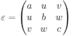
- The default is the identity matrix (a = b = c = 1 and u = v = w = 0).
-
mu[number] - The (frequency-independent) isotropic relative permeability μ. Default value = 1. Using
(mu μ)is actually a synonym for(mu-diag μ μ μ). -
mu-diagandmu-offdiag[vector3] - These properties allow you to specify μ as an arbitrary real-symmetric tensor, by giving the diagonal and offdiagonal parts exactly as for ε above, again defaulting to the identity matrix.
-
D-conductivity[number] - The (frequency-independent) electric conductivity σD. Default value = 0. You can also specify an diagonal anisotropic conductivity tensor by using the property
D-conductivity-diag[vector3], which takes three numbers or a vector3 to give the σD tensor diagonal. See also Conductivity in Meep. -
B-conductivity[number] - The (frequency-independent) magnetic conductivity σB. Default value = 0. You can also specify an diagonal anisotropic conductivity tensor by using the property
B-conductivity-diag[vector3], which takes three numbers or a vector3 to give the σB tensor diagonal. See also Conductivity in Meep. -
chi2[number] - The nonlinear (Pockels) susceptibility χ(2). Default value = 0. See also Nonlinearity in Meep.
-
chi3[number] - The nonlinear (Kerr) susceptibility χ(3). Default value = 0. (See e.g. Meep Tutorial/Third harmonic generation.) See also Nonlinearity in Meep.
-
E-susceptibilities[list ofsusceptibilityclass] - List of dispersive susceptibilities (see below) added to the dielectric constant ε, in order to model material dispersion; defaults to none. (See e.g. Meep Tutorial/Material dispersion.) See also Material dispersion in Meep. For backwards compatibility, synonyms of
E-susceptibilitiesareE-polarizationsandpolarizations. -
H-susceptibilities[list ofsusceptibilityclass] - List of dispersive susceptibilities (see below) added to the permeability μ, in order to model material dispersion; defaults to none. (See e.g. Meep Tutorial/Material dispersion.) See also Material dispersion in Meep. For backwards compatibility, a synonym of
H-susceptibilitiesisH-polarizations.
-
-
perfect-metal - A perfectly conducting metal; this class has no properties and you normally just use the predefined
metalobject, above. (To model imperfect conductors, use a dispersive dielectric material.) See also the predefined variablesmetal,perfect-electric-conductor, andperfect-magnetic-conductorabove. -
material-function - This material type allows you to specify the material as an arbitrary function of position. It has one property:
-
material-func[function] - A function of one argument, the position
vector3, that returns the material at that point. Note that the function you supply can return any material; wild and crazy users could even return anothermaterial-functionobject (which would then have its function invoked in turn).- Instead of
material-func, you can useepsilon-func: forepsilon-func, you give it a function of position that returns the dielectric constant at that point.
- Instead of
- Important: If your material function returns nonlinear, dispersive (Lorentzian or conducting), or magnetic materials, you should also include a list of these materials in the
extra-materialsinput variable (above) to let Meep know that it needs to support these material types in your simulation. (For dispersive materials, you need to include a material with the same γn and ωn values, so you can only have a finite number of these, whereas σn can vary continuously if you want and a matching σn need not be specified inextra-materials. For nonlinear or conductivity materials, yourextra-materialslist need not match the actual values of σ or χ returned by your material function, which can vary continuously if you want.)
-
Complex ε and μ: you cannot specify a frequency-independent complex ε or μ in Meep (where the imaginary part is a frequency-independent loss), but there is an alternative. That is because there are only two important physical situations. First, if you only care about the loss in a narrow bandwidth around some frequency, you can set the loss at that frequency via the conductivity (see Conductivity in Meep). Second, if you care about a broad bandwidth, then all physical materials have a frequency-dependent imaginary (and real) ε (and/or μ), and you need to specify that frequency dependence by fitting to Lorentzian (and/or Drude) resonances via the lorentzian-susceptibility (or drude-susceptibility) classes below.
Dispersive dielectric (and magnetic) materials, above, are specified via a list of objects that are subclasses of type susceptibility.
-
susceptibility - Parent class for various dispersive susceptibility terms, parameterized by an anisotropic amplitude σ (see Material dispersion in Meep):
-
sigma[number] - The scale factor σ. You can also specify an anisotropic σ tensor by using the property
sigma-diag[vector3], which takes three numbers or a vector3 to give the σn tensor diagonal, andsigma-offdiag[vector3] which specifies the offdiagonal elements (defaults to 0). That is,(sigma-diag a b c)and(sigma-offdiag u v w)corresponds to a σ tensor 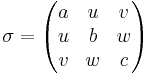
-
-
lorentzian-susceptibility - Specifies a single dispersive susceptibility of Lorentzian (damped harmonic oscillator) form (see Material dispersion in Meep), with the parameters (in addition to σ):
-
frequency[number] - The resonance frequency fn = ωn / 2π.
-
gamma[number] - The resonance loss rate γn / 2π.
-
-
drude-susceptibility - Specifies a single dispersive susceptibility of Drude form (see Material dispersion in Meep), with the parameters (in addition to σ):
-
frequency[number] - The frequency scale factor fn = ωn / 2π which multiplies σ (not a resonance frequency).
-
gamma[number] - The loss rate γn / 2π.
-
Meep also supports a somewhat unusual polarizable medium, a Lorentzian susceptibility with a random noise term added into the damped-oscillator equation at each point. This can be used to directly model thermal radiation in both the far field (as described in Luo et al., 2004) and the near field (as described in Rodriguez et al., 2011). (Note, however that it is more efficient to compute far-field thermal radiation using Kirchhoff's law of radiation, which states that emissivity equals absorptivity. Near-field thermal radiation can usually be computed more efficiently using frequency domain techniques, e.g. via our SCUFF-EM code, as described by Rodriguez et al., 2013.)
-
noisy-lorentzian-susceptibilityornoisy-drude-susceptibility - Specifies a single dispersive susceptibility of Lorentzian (damped harmonic oscillator) or Drude form (see Material dispersion in Meep), with the same σ,
frequency, andgamma) parameters, but with an additional Gaussian random noise term (uncorrelated in space and time, zero mean) added to the P damped-oscillator equation.-
noise-amp[number] - The noise has root-mean square amplitude σ⋅
noise-amp.
-
geometric-object
This class, and its descendants, are used to specify the solid geometric objects that form the dielectric structure being simulated. The base class is:
-
geometric-object - Properties:
-
material[material-typeclass] - The material that the object is made of (usually some sort of dielectric). No default value (must be specified).
-
center[vector3] - Center point of the object. No default value.
-
One normally does not create objects of type geometric-object directly, however; instead, you use one of the following subclasses. Recall that subclasses inherit the properties of their superclass, so these subclasses automatically have the material and center properties (which must be specified, since they have no default values).
In a two-dimensional calculation, only the intersections of the objects with the x-y plane are considered.
-
sphere - A sphere. Properties:
-
radius[number] - Radius of the sphere. No default value.
-
-
cylinder - A cylinder, with circular cross-section and finite height. Properties:
-
radius[number] - Radius of the cylinder's cross-section. No default value.
-
height[number] - Length of the cylinder along its axis. No default value.
-
axis[vector3] - Direction of the cylinder's axis; the length of this vector is ignored. Defaults to point parallel to the z axis.
-
-
cone - A cone, or possibly a truncated cone. This is actually a subclass of
cylinder, and inherits all of the same properties, with one additional property. The radius of the base of the cone is given by theradiusproperty inherited fromcylinder, while the radius of the tip is given by the new property,radius2. (Thecenterof a cone is halfway between the two circular ends.)-
radius2[number] - Radius of the tip of the cone (i.e. the end of the cone pointed to by the
axisvector). Defaults to zero (a "sharp" cone).
-
-
block - A parallelepiped (i.e., a brick, possibly with non-orthogonal axes). Properties:
-
size[vector3] - The lengths of the block edges along each of its three axes. Not really a 3-vector, but it has three components, each of which should be nonzero. No default value.
-
e1,e2,e3[vector3] - The directions of the axes of the block; the lengths of these vectors are ignored. Must be linearly independent. They default to the three lattice directions.
-
-
ellipsoid - An ellipsoid. This is actually a subclass of
block, and inherits all the same properties, but defines an ellipsoid inscribed inside the block.
Here are some examples of geometric objects created using the above classes, assuming mat is some material we have defined:
; A cylinder of infinite radius and height 0.25 pointing along the x axis,
; centered at the origin:
(make cylinder (center 0 0 0) (material mat)
               (radius infinity) (height 0.25) (axis 1 0 0))
; An ellipsoid with its long axis pointing along (1,1,1), centered on
; the origin (the other two axes are orthogonal and have equal
; semi-axis lengths):
(make ellipsoid (center 0 0 0) (material mat)
                (size 0.8 0.2 0.2)
               (e1 1 1 1)
               (e2 0 1 -1)
               (e3 -2 1 1))
; A unit cube of material m with a spherical air hole of radius 0.2 at
; its center, the whole thing centered at (1,2,3):
(set! geometry (list
               (make block (center 1 2 3) (material mat) (size 1 1 1))
               (make sphere (center 1 2 3) (material air) (radius 0.2))))
symmetry
This class is used for the symmetries input variable, to specify symmetries (which must preserve both the structure and the sources) for Meep to exploit. Any number of symmetries can be exploited simultaneously, but there is no point in specifying redundant symmetries: the computational cell can be reduced by at most a factor of 4 in 2d and 8 in 3d. See also Exploiting symmetry in Meep.
-
symmetry - A single symmetry to exploit. This is the base class of the specific symmetries below, so normally you don't create it directly. However, it has two properties which are shared by all symmetries:
-
direction[directionconstant] - The direction of the symmetry (the normal to a mirror plane or the axis for a rotational symmetry). e.g.
X,Y, ... (only Cartesian/grid directions are allowed). No default value. -
phase[cnumber] - An additional phase to multiply the fields by when operating the symmetry on them; defaults to
1.0. e.g. a phase of-1for a mirror plane corresponds to an odd mirror. (Technically, you are essentially specifying the representation of the symmetry group that your fields and sources transform under.)
-
The specific symmetry sub-classes are:
-
mirror-sym - A mirror symmetry plane. Here, the
directionis the direction normal to the mirror plane. -
rotate2-sym - A 180° (twofold) rotational symmetry (a.k.a. C2). Here, the
directionis the axis of the rotation. -
rotate4-sym - A 90° (fourfold) rotational symmetry (a.k.a. C4). Here, the
directionis the axis of the rotation.
pml
This class is used for specifying the PML absorbing boundary layers around the cell, if any, via the pml-layers input variable. See also Perfectly matched layers. pml-layers can be zero or more pml objects, with multiple objects allowing you to specify different PML layers on different boundaries.
-
pml - A single PML layer specification, which sets up one or more PML layers around the boundaries according to the following properties.
-
thickness[number] - The spatial thickness of the PML layer (which extends from the boundary towards the inside of the computational cell). The thinner it is, the more numerical reflections become a problem. No default value.
-
direction[directionconstant] - Specify the direction of the boundaries to put the PML layers next to. e.g. if
X, then specifies PML on the boundaries (depending on the value of
 side, below). Default is the special valueALL, which puts PML layers on the boundaries in all directions. -
side[boundary-sideconstant] - Specify which side,
LoworHighof the boundary or boundaries to put PML on. e.g. if side isLowand direction isX, then a PML layer is added to the − x boundary. Default is the special valueALL, which puts PML layers on both sides. -
strength[number] - A strength (default is
1.0) to multiply the PML absorption coefficient by. A strength of2.0will square the theoretical asymptotic reflection coefficient of the PML (making it smaller), but will also increase numerical reflections. Alternatively, you can changeR-asymptotic, below. -
R-asymptotic[number] - The asymptotic reflection in the limit of infinite resolution or infinite PML thickness, for refections from air (an upper bound for other media with index > 1). (For a finite resolution or thickness, the reflection will be much larger, due to the discretization of Maxwell's equation.) The default value is 10−15, which should suffice for most purposes. (You want to set this to be small enough so that waves propagating within the PML are attenuated sufficiently, but making
R-asymptotictoo small will increase the numerical reflection due to discretization.) -
pml-profile[function] - By default, Meep turns on the PML conductivity quadratically within the PML layer—one doesn't want to turn it on suddenly, because that exacerbates reflections due to the discretization. More generally, with
pml-profileone can specify an arbitrary PML "profile" function f(u) that determines the shape of the PML absorption profile up to an overall constant factor. u goes from 0 to 1 at the start and end of the PML, and the default is f(u)=u2. In some cases where a very thick PML is required, such as in a periodic medium (where there is technically no such thing as a true PML, only a pseudo-PML), it can be advantageous to turn on the PML absorption more smoothly (see Oskooi et al., 2008). For example, one can use a cubic profile f(u)=u3 by specifying(pml-profile (lambda (u) (* u u u))).
-
absorber
Instead of a pml layer, there is an alternative class called absorber which is a drop-in replacement for pml. For example, you can do (set! pml-layers (list (make absorber (thickness 2)))) instead of (set! pml-layers (list (make pml (thickness 2)))). All the parameters are the same as for pml, above. You can have a mix of pml on some boundaries and absorber on others.
The absorber class does not implement a perfectly matched layer (PML), however (except in 1d). Instead, it is simply a scalar electric and magnetic conductivity that turns on gradually within the layer according to the pml-profile (defaulting to quadratic). Such a scalar conductivity gradient is only reflectionless in the limit as the layer becomes sufficiently thick.
The main reason to use absorber is if you have a case in which PML fails:
- No true PML exists for periodic media, and a scalar absorber is cheaper and is generally just as good. See Oskooi et al. (2008).
- PML can lead to divergent fields for certain waveguides with "backward-wave" modes; this can easily happen in metallic with surface plasmons, and a scalar absorber is your only choice. See Loh et al. (2009).
- PML can fail if you have a waveguide hitting the edge of your computational cell at an angle. See Oskooi et. al. (2011).
source
The source class is used to specify the current sources (via the sources input variable). Note that all sources in Meep are separable in time and space, i.e. of the form 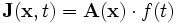 for some functions
  and f. (Non-separable sources can be simulated, however, by modifying the sources after each time step.) When real fields are being used (which is the default in many cases...see the
 force-complex-fields? input variable), only the real part of the current source is used by Meep.
Important note: These are current sources (J terms in Maxwell's equations), even though they are labelled by electric/magnetic field components. They do not specify a particular electric/magnetic field (which would be what is called a "hard" source in the FDTD literature). There is no fixed relationship between the current source and the resulting field amplitudes; it depends on the surrounding geometry, as described in the Meep FAQ and in our book chapter online.
-
source - The source class has the following properties:
-
src[src-timeclass] - Specify the time-dependence of the source (see below). No default.
-
component[componentconstant] - Specify the direction and type of the current component: e.g.
Ex,Ey, etcetera for an electric-charge current, andHx,Hy, etcetera for a magnetic-charge current. Note that currents pointing in an arbitrary direction are specified simply as multiple current sources with the appropriate amplitudes for each component. No default. center[vector3]- The location of the center of the current source in the computational cell; no default.
size[vector3]- The size of the current distribution along each direction of the computational cell. The default is (0,0,0): a point-dipole source.
amplitude[cnumber]- An overall (complex) amplitude multiplying the the current source. Default is
1.0. amp-func[function]- A Scheme function of a single argument, that takes a vector3 giving a position and returns a (complex) current amplitude for that point. The position argument is relative to the
centerof the current source, so that you can move your current around without changing your function. The default is'()(null), meaning that a constant amplitude of 1.0 is used. Note that your amplitude function (if any) is multiplied by theamplitudeproperty, so both properties can be used simultaneously.
-
As described in section 4.2 of our book chapter online, it is also possible to supply a source that is designed to couple exclusively into a single waveguide mode (or other mode of some cross section or periodic region) at a single frequency, and which couples primarily into that mode as long as the bandwidth is not too broad. This is possible if you have MPB (version 1.5 or later) installed: Meep will call MPB to compute the field profile of the desired mode, and uses the field profile to produce an equivalent current source. (Note: this feature does not work in cylindrical coordinates.) To do this, instead of a source you should use an eigenmode-source:
-
eigenmode-source - This is a subclass of
sourceand has all of the properties ofsourceabove. However, you normally do not specify acomponent. Instead ofcomponent, the current source components and amplitude profile are computed by calling MPB to compute the modes of the dielectric profile in the region given by thesizeandcenterof the source, with the modes computed as if the source region were repeated periodically in all directions. (If anamplitudeand/oramp-funcare supplied, they are multiplied by this current profile.) The desired eigenmode and other features are specified by the following properties:-
eig-band[integer] - The index n (1,2,3,...) of the desired band ωn(k) to compute in MPB (1 denotes the lowest-frequency band at a given k point, and so on).
-
direction[X,Y, orZ; defaultAUTOMATIC],eig-match-freq?[boolean; defaulttrue],eig-kpoint[vector3] - By default (if
eig-match-freq?istrue), Meep tries to find a mode with the same frequency ωn(k) as thesrcproperty (above), by scanning k vectors in the givendirection(using MPB's find-k functionality; alternatively, ifeig-kpointis supplied, it is used as an initial guess and direction for k ). By default,directionis the direction normal to the source region, assumingsizeis d–1 dimensional in a d-dimensional simulation (e.g. a plane in 3d). Alternatively (ifeig-match-freq?isfalse), you can specify a particular k vector of the desired mode witheig-kpoint(in Meep units of 2π/a). -
eig-parity[NO-PARITY(= default),EVEN-Z(=TE),ODD-Z(=TM),EVEN-Y,ODD-Y] - The parity (= polarization in 2d) of the mode to calculate, assuming the structure has z and/or y mirror symmetry in the source region. If the structure has both y and z mirror symmetry, you can combine more than one of these, e.g.
EVEN-Z + ODD-Y. The default isNO-PARITY, in which case MPB computes all of the bands (which will still be even or odd if the structure has mirror symmetry, of course). This is especially useful in 2d simulations to restrict yourself to a desired polarization. -
eig-resolution[integer, defaults to same as Meep resolution] - The spatial resolution to use in MPB for the eigenmode calculations. This defaults to the same resolution as Meep, but you can use a higher resolution (in which case the structure is linearly interpolated from the Meep pixels).
-
eig-tolerance[number, defaults to 10–7] - The tolerance to use in the MPB eigensolver. (MPB terminates when the eigenvalues stop changing to less than this fractional tolerance.)
-
component[as above, but defaults toALL-COMPONENTS] - Once the MPB modes are computed, equivalent electric and magnetic sources are created within Meep. By default, these sources include magnetic and electric currents in all transverse directions within the source region, corresponding to the mode fields as described in our book chapter. If you specify a
componentproperty, however, you can include only one component of these currents if you wish. Most people won't need this feature. -
eig-lattice-size[vector3],eig-lattice-center[vector3] - Normally, the MPB computational unit cell is the same as the source volume (given by the
sizeandcenterparameters). However, occasionally you want the unit cell to be larger than the source volume. For example, to create an eigenmode source in a periodic medium (photonic crystal), you need to pass MPB the entire unit cell of the periodic medium, but once the mode is computed then the actual current sources need only lie on a cross section of that medium. To accomplish this, you can specify the optionaleig-lattice-sizeandeig-lattice-center, which define a volume (which must enclosesizeandcenter) that is used for the unit cell in MPB (with the dielectric function ε taken from the corresponding region in the Meep simulation).
-
Note that MPB only supports dispersionless non-magnetic materials (but it does support anisotropic ε). Any nonlinearities, magnetic responses µ, conductivities σ, or dispersive polarizations in your materials will be ignored when computing the eigenmode source. PML will also be ignored.
The src-time object, which specifies the time dependence of the source, can be one of the following three classes.
-
continuous-src - A continuous-wave source proportional to exp( − iωt), possibly with a smooth (exponential/tanh) turn-on/turn-off. It has the properties:
frequency[number]- The frequency f in units of c/distance (or ω in units of 2πc/distance) (see Units in Meep). No default value. You can instead specify
(wavelength x)or(period x), which are both a synonym for(frequency (/ 1 x)); i.e. 1/ω in these units is the vacuum wavelength or the temporal period. start-time[number]- The starting time for the source; default is
0(turn on at t = 0). end-time[number]- The end time for the source; default is
infinity(never turn off). width[number]- Roughly, the temporal width of the smoothing (technically, the inverse of the exponential rate at which the current turns off and on). Default is
0(no smoothing). You can instead specify(fwidth x), which is a synonym for(width (/ 1 x))(i.e. the frequency width is proportional to the inverse of the temporal width). cutoff[number]- How many
widths the current decays for before we cut it off and set it to zero; the default is3.0. A larger value ofcutoffwill reduce the amount of high-frequency components that are introduced by the start/stop of the source, but will of course lead to longer simulation times.
-
gaussian-src - A Gaussian-pulse source roughly proportional to exp( − iωt − (t − t0)2 / 2w2). Technically, the "Gaussian" sources in Meep are the (discrete-time) derivative of a Gaussian, i.e. they are
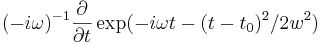 , but the difference between this and a true Gaussian is usually irrelevant. It has the properties:
frequency[number]- The center frequency f in units of c/distance (or ω in units of 2πc/distance) (see Units in Meep). No default value. You can instead specify
(wavelength x)or(period x), which are both a synonym for(frequency (/ 1 x)); i.e. 1/ω in these units is the vacuum wavelength or the temporal period. width[number]- The width w used in the Gaussian. No default value. You can instead specify
(fwidth x), which is a synonym for(width (/ 1 x))(i.e. the frequency width is proportional to the inverse of the temporal width). start-time[number]- The starting time for the source; default is
0(turn on at t = 0). (Not the time of the peak! See below.) cutoff[number]- How many
widths the current decays for before we cut it off and set it to zero—this applies for both turn-on and turn-off of the pulse. The default is5.0. A larger value ofcutoffwill reduce the amount of high-frequency components that are introduced by the start/stop of the source, but will of course lead to longer simulation times. The peak of the gaussian is reached at the time t0=start-time+cutoff*width.
-
custom-src - A user-specified source function f(t). You can also specify start/end times (at which point your current is set to zero whether or not your function is actually zero). These are optional, but you must specify an
end-timeexplicitly if you want functions likerun-sourcesto work, since they need to know when your source turns off.-
src-func[function] - The function f(t) specifying the time-dependence of the source. It should take one argument (the time in Meep units) and return a complex number.
start-time[number]- The starting time for the source; default is
(- infinity)(turn on at ). Note, however, that the simulation normally starts at t = 0 with zero fields as the initial condition, so there is implicitly a sharp turn-on at t = 0 whether you specify it or not.
end-time[number]- The end time for the source; default is
infinity(never turn off).
-
flux-region
A flux-region object is used with add-flux below to specify a region in which Meep should accumulate the appropriate Fourier-transformed fields in order to compute a flux spectrum.
flux-region- A region (volume, plane, line, or point) in which to compute the integral of the Poynting vector of the Fourier-transformed fields. Its properties are:
center[vector3]- The center of the flux region (no default).
size[vector3]- The size of the flux region along each of the coordinate axes; default is (0,0,0) (a single point).
direction[directionconstant]- The direction in which to compute the flux (e.g.
X,Y, etcetera). The default isAUTOMATIC, in which the direction is determined by taking the normal direction if the flux region is a plane (or a line, in 2d). If the normal direction is ambiguous (e.g. for a point or volume), then you must specify thedirectionexplicitly (not doing so will lead to an error). weight[cnumber]- A weight factor to multiply the flux by when it is computed; default is
1.0.
Note that the flux is always computed in the positive coordinate direction, although this can effectively be flipped by using a weight of -1.0. (This is useful, for example, if you want to compute the outward flux through a box, so that the sides of the box add instead of subtract!)
Miscellaneous functions
Here, we describe a number of miscellaneous useful functions provided by Meep.
See also the reference section of the libctl manual, which describes a number of useful functions defined by libctl.
Geometry utilities
Some utility functions are provided to help you manipulate geometric objects:
-
(shift-geometric-object obj shift-vector) - Translate
objby the 3-vectorshift-vector. -
(geometric-object-duplicates shift-vector min-multiple max-multiple obj) - Return a list of duplicates of
obj, shifted by various multiples ofshift-vector(frommin-multipletomax-multiple, inclusive, in steps of 1). -
(geometric-objects-duplicates shift-vector min-multiple max-multiple obj-list) - Same as
geometric-object-duplicates, except operates on a list of objects,obj-list. If A appears before B in the input list, then all the duplicates of A appear before all the duplicates of B in the output list. -
(geometric-objects-lattice-duplicates obj-list [ ux uy uz ]) - Duplicates the objects in
obj-listby multiples of the Cartesian basis vectors, making all possible shifts of the "primitive cell" (see below) that fit inside the lattice cell. (This is useful for supercell calculations; see the [user-tutorial.html tutorial].) The primitive cell to duplicate isuxbyuybyuz, in units of the Cartesian basis vectors. These three parameters are optional; any that you do not specify are assumed to be1. -
(point-in-object? point obj) - Returns whether or not the given 3-vector
pointis inside the geometric objectobj. -
(point-in-periodic-object? point obj) - As
point-in-object?, but also checks translations of the given object by the lattice vectors. -
(display-geometric-object-info indent-by obj) - Outputs some information about the given
obj, indented byindent-byspaces.
Output file names
The output file names used by Meep, e.g. for HDF5 files, are automatically prefixed by the input variable filename-prefix. If filename-prefix is "" (the default), however, then Meep constructs a default prefix based on the current ctl file name with ".ctl" replaced by "-": e.g. tst.ctl implies a prefix of "tst-". You can get this prefix by running:
(get-filename-prefix)- Return the current prefix string that is prepended, by default, to all file names.
If you don't want to use any prefix, then you should set filename-prefix to false.
In addition to the filename prefix, you can also specify that all the output files be written into a newly-created directory (if it does not yet exist). This is done by running:
(use-output-directory [dirname])- Put output in a subdirectory, which is created if necessary. If the optional argument dirname is specified, that is the name of the directory. Otherwise, the directory name is the current ctl file name with
".ctl"replaced by"-out": e.g.tst.ctlimplies a directory of"tst-out".
Misc.
(volume (center ...) (size ...))- Many Meep functions require you to specify a volume in space, corresponding to the C++ type
meep::geometric_volume. This function creates such a volume object, given thecenterandsizeproperties (just like e.g. ablockobject). If thesizeis not specified, it defaults to (0,0,0), i.e. a single point. (meep-time)- Return the current simulation time (in simulation time units, not wall-clock time!). (e.g. during a run function.)
- Occasionally, e.g. for termination conditions of the form time < T?, it is desirable to round the time to single precision in order to avoid small differences in roundoff error from making your results different by one timestep from machine to machine (a difference much bigger than roundoff error); in this case you can call
(meep-round-time)instead, which returns the time rounded to single precision.
Field computations
Meep supports a large number of functions to perform computations on the fields. Currently, most of them are accessed via the lower-level C++/SWIG interface, but we are slowly adding simpler, higher-level versions of them here.
(get-field-point c pt)- Given a
componentorderived-componentconstantcand avector3pt, returns the value of that component at that point. (get-epsilon-point pt)- Equivalent to
(get-field-point Dielectric pt). (flux-in-box dir box)- Given a
directionconstant, and ameep::volume*, returns the flux (the integral of![\Re [\mathbf{E}^* \times \mathbf{H}]](/wiki/images/math/d/f/5/df5da403fca9de978b2fa3e687a18286.png) ) in that volume. Most commonly, you specify a volume that is a plane or a line, and a direction perpendicular to it, e.g.
) in that volume. Most commonly, you specify a volume that is a plane or a line, and a direction perpendicular to it, e.g. (flux-in-box X (volume (center 0) (size 0 1 1))). (electric-energy-in-box box)- Given a
meep::volume*, returns the integral of the electric-field energy in the given volume. (If the volume has zero size along a dimension, a lower-dimensional integral is used.)
(magnetic-energy-in-box box)- Given a
meep::volume*, returns the integral of the magnetic-field energyin the given volume. (If the volume has zero size along a dimension, a lower-dimensional integral is used.)
(field-energy-in-box box)- Given a
meep::volume*, returns the integral of the electric+magnetic-field energy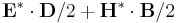 in the given volume. (If the volume has zero size along a dimension, a lower-dimensional integral is used.)
Note that if you are at a fixed frequency and you use complex fields (Bloch-periodic boundary conditions or fields-complex?=true), then one half of the flux or energy integrals above corresponds to the time-average of the flux or energy for a simulation with real fields.
Often, you want the integration box to be the entire computational cell. A useful function to return this box, which you can then use for the box arguments above, is (meep-fields-total-volume fields), where fields is the global variable (above) holding the current meep::fields object.
One powerful feature is that you can supply an arbitrary function  of position
  and various field components
  and ask Meep to integrate it over a given volume, find its maximum, or output it (via
 output-field-function, described later). This is done via the functions:
(integrate-field-function cs func [where] [fields-var])- Returns the integral of the complex-valued function
funcover themeep::geometric_volumespecified bywhere(defaults to entire computational cell) for themeep::fieldsspecified byfields-var(defaults tofields).funcis a function of position (avector3, its first argument) and zero or more field components specified bycs: a list ofcomponentconstants.funccan be real- or complex-valued. - (If any dimension of
whereis zero, that dimension is not integrated over. In this way you can specify one-, two-, or three-dimensional integrals.) (max-abs-field-function cs func [where] [fields-var])- As
integrate-field-function, but returns the maximum absolute value offuncin the volumewhereinstead of its integral.
(The integration is performed by summing over the grid points with a simple trapezoidal rule, and the maximum is similarly over the grid points.) See also Meep field-function examples for illustrations of how to call integrate-field-function and max-abs-field-function. See also Synchronizing the magnetic and electric fields if you want to do computations combining the electric and magnetic fields.
Occasionally, one wants to compute an integral that combines fields from two separate simulations (e.g. for nonlinear coupled-mode calculations). This functionality is supported in Meep, as long as the two simulations have the same computational cell, the same resolution, the same boundary conditions and symmetries (if any), and the same PML layers (if any).
(integrate2-field-function fields2 cs1 cs2 func [where] [fields-var])- Similar to
integrate-field-function, but takes additional parametersfields2andcs2.fields2is ameep::fields*object similar to the globalfieldsvariable (see below) specifying the fields from another simulation.cs1is a list of components to integrate with fromfields-var(defaults tofields), as forintegrate-field-function, whilecs2is a list of components to integrate fromfields2. Similar tointegrate-field-function,funcis a function that returns an number given arguments consisting of: the position vector, followed by the values of the components specified bycs1(in order), followed by the values of the components specified bycs2(in order).
To get two fields in memory at once for integrate2-field-function, the easiest way is to run one simulation within a given .ctl file, then save the results in another fields variable, then run a second simulation. This would look something like:
...set up and run first simulation...
(define fields2 fields) ; save the fields in a variable
(set! fields '()) ; prevent the fields from getting deallocated by reset-meep
(reset-meep)
...set up and run second simulation...
It is also possible to timestep both fields simultaneously (e.g. doing one timestep of one simulation then one timestep of another simulation, and so on, but this requires you to call much lower-level functions like (meep-fields-step fields).
Reloading parameters
Once the fields/simulation have been initialized, you can change the values of various parameters by using the following functions:
(reset-meep)- Reset all of Meep's parameters, deleting the fields, structures, etcetera, from memory as if you had not run any computations.
(restart-fields)- Restart the fields at time zero, with zero fields. (Does not reset the Fourier transforms of the flux planes, which continue to be accumulated.)
(change-k-point! k)- Change the
k-point(the Bloch periodicity). (change-sources! new-sources)- Change the
sourcesinput variable tonew-sources, and changes the sources used for the current simulation.
(More to come...)
Flux spectra
Given a bunch of flux-region objects (see above), you can tell Meep to accumulate the Fourier transforms of the fields in those regions in order to compute flux spectra. See also the transmission/reflection spectra introduction and the Meep tutorial. The most important function is:
(add-flux fcen df nfreq flux-regions...)- Add a bunch of
flux-regions to the current simulation (initializing the fields if they have not yet been initialized), telling Meep to accumulate the appropriate field Fourier transforms fornfreqequally spaced frequencies covering the frequency rangefcen-df/2tofcen+df/2. Return a flux object, which you can pass to the functions below to get the flux spectrum, etcetera.
As described in the tutorial, you normally use add-flux via statements like:
(define transmission (add-flux ...))
to store the flux object in a variable. add-flux initializes the fields if necessary, just like calling run, so you should only call it after setting up your geometry, sources, pml-layers, etcetera. You can create as many flux objects as you want, e.g. to look at powers flowing in different regions or in different frequency ranges. Note, however, that Meep has to store (and update at every time step) a number of Fourier components equal to the number of grid points intersecting the flux region multiplied by the number of electric and magnetic field components required to get the Poynting vector multiplied by nfreq, so this can get quite expensive (in both memory and time) if you want a lot of frequency points over large regions of space.
Once you have called add-flux, the Fourier transforms of the fields are accumulated automatically during time-stepping by the run functions. At any time, you can ask for Meep to print out the current flux spectrum via:
(display-fluxes fluxes...)- Given a number of flux objects, this displays a comma-separated table of frequencies and flux spectra, prefixed by "flux1:" or similar (where the number is incremented after each run). All of the fluxes should be for the same
fcen/df/nfreq. The first column are the frequencies, and subsequent columns are the flux spectra.
You might have to do something lower-level if you have multiple flux regions corresponding to different frequency ranges, or have other special needs. (display-fluxes f1 f2 f3) is actually equivalent to (display-csv "flux" (get-flux-freqs f1) (get-fluxes f1) (get-fluxes f2) (get-fluxes f3), where display-csv takes a bunch of lists of numbers and prints them as a comma-separated table, and we are calling two lower-level functions:
(get-flux-freqs flux)- Given a flux object, returns a list of the frequencies that it is computing the spectrum for.
(get-fluxes flux)- Given a flux object, returns a list of the current flux spectrum that it has accumulated.
As described in the Meep tutorial, for a reflection spectrum you often want to save the Fourier-transformed fields from a "normalization" run and then load them into another run to be subtracted. This can be done via:
(save-flux filename flux)- Save the Fourier-transformed fields corresponding to the given flux object in an HDF5 file of the given name (without the ".h5" suffix) (the current filename-prefix is prepended automatically).
(load-flux filename flux)- Load the Fourier-transformed fields into the given flux object (replacing any values currently there) from an HDF5 file of the given name (without the ".h5" suffix) (the current filename-prefix is prepended automatically). You must load from a file that was saved by
save-fluxin a simulation of the same dimensions (for both the computational cell and the flux regions) with the same number of processors. (load-minus-flux filename flux)- As
load-flux, but negates the Fourier-transformed fields after they are loaded. This means that they will be subtracted from any future field Fourier transforms that are accumulated. (scale-flux-fields s flux)- Scale the Fourier-transformed fields in
fluxby the complex numbers. e.g.load-minus-fluxis equivalent toload-fluxfollowed byscale-flux-fieldswiths=-1.
Force spectra
Very similar to flux spectra, you can also compute force spectra: forces on an object as a function of frequency, computed by Fourier transforming the fields and integrating the vacuum Maxwell stress tensor
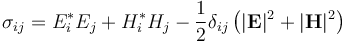
over a surface S via 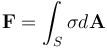 . We recommend that you normally only evaluate the stress tensor over a surface lying in vacuum, as the interpretation and definition of the stress tensor in arbitrary media is often problematic (the subject of extensive and controversial literature). (It is fine if the surface encloses an object made of arbitrary materials, as long as the surface itself is in vacuum.)
See also the optical forces Meep tutorial.
Most commonly, you will want to normalize the force spectrum in some way, just as for flux spectra. Most simply, you could divide two different force spectra to compute the ratio of forces on two objects. Often, you will divide a force spectrum by a flux spectrum, to divide the force F by the incident power P on an object, in order to compute the useful dimensionless ratio Fc/P (where c=1 in Meep units). For example, it is a simple exercise to show that the force F on a perfectly reflecting mirror with normal-incident power P satisfies Fc/P=2, and for a perfectly absorbing (black) surface Fc/P=1.
The usage is similar to the flux spectra: you define a set of force-region objects telling Meep where it should compute the Fourier-transformed fields and stress tensors, and call add-force to add these regions to the current simulation over a specified frequency bandwidth, and then use display-forces to display the force spectra at the end. There are also save-force, load-force, and load-minus-force functions that you can use to subtract the fields from two simulation, e.g. in order to compute just the force from scattered fields, similar to the flux spectra. These types and functions are defined as follows:
force-region- A region (volume, plane, line, or point) in which to compute the integral of the stress tensor of the Fourier-transformed fields. Its properties are:
center[vector3]- The center of the force region (no default).
size[vector3]- The size of the force region along each of the coordinate axes; default is (0,0,0) (a single point).
direction[directionconstant]- The direction of the force that you wish to compute (e.g.
X,Y, etcetera). Unlikeflux-region, you must specify this explicitly, because there is not generally any relationship between the direction of the force and the orientation of the force region. weight[cnumber]- A weight factor to multiply the force by when it is computed; default is
1.0.
In most circumstances, you should define a set of force-regions whose union is a closed surface (lying in vacuum and enclosing the object that is experiencing the force).
(add-force fcen df nfreq force-regions...)- Add a bunch of
force-regions to the current simulation (initializing the fields if they have not yet been initialized), telling Meep to accumulate the appropriate field Fourier transforms fornfreqequally spaced frequencies covering the frequency rangefcen-df/2tofcen+df/2. Return a force object, which you can pass to the functions below to get the force spectrum, etcetera.
As for flux regions, you normally use add-force via statements like:
(define Fx (add-force ...))
to store the flux object in a variable. add-force initializes the fields if necessary, just like calling run, so you should only call it after setting up your geometry, sources, pml-layers, etcetera. You can create as many force objects as you want, e.g. to look at forces on different objects, in different directions, or in different frequency ranges. Note, however, that Meep has to store (and update at every time step) a number of Fourier components equal to the number of grid points intersecting the force region, multiplied by the number of electric and magnetic field components required to get the stress vector, multiplied by nfreq, so this can get quite expensive (in both memory and time) if you want a lot of frequency points over large regions of space.
Once you have called add-force, the Fourier transforms of the fields are accumulated automatically during time-stepping by the run functions. At any time, you can ask for Meep to print out the current force spectrum via:
(display-forces forces...)- Given a number of force objects, this displays a comma-separated table of frequencies and force spectra, prefixed by "force1:" or similar (where the number is incremented after each run). All of the forces should be for the same
fcen/df/nfreq. The first column are the frequencies, and subsequent columns are the force spectra.
You might have to do something lower-level if you have multiple force regions corresponding to different frequency ranges, or have other special needs. (display-forces f1 f2 f3) is actually equivalent to (display-csv "force" (get-force-freqs f1) (get-forces f1) (get-forces f2) (get-forces f3), where display-csv takes a bunch of lists of numbers and prints them as a comma-separated table, and we are calling two lower-level functions:
(get-force-freqs flux)- Given a force object, returns a list of the frequencies that it is computing the spectrum for.
(get-forces flux)- Given a force object, returns a list of the current force spectrum that it has accumulated.
As described in the Meep tutorial, to compute the force from scattered fields often want to save the Fourier-transformed fields from a "normalization" run and then load them into another run to be subtracted. This can be done via:
(save-force filename force)- Save the Fourier-transformed fields corresponding to the given force object in an HDF5 file of the given name (without the ".h5" suffix) (the current filename-prefix is prepended automatically).
(load-force filename force)- Load the Fourier-transformed fields into the given force object (replacing any values currently there) from an HDF5 file of the given name (without the ".h5" suffix) (the current filename-prefix is prepended automatically). You must load from a file that was saved by
save-forcein a simulation of the same dimensions (for both the computational cell and the force regions) with the same number of processors. (load-minus-force filename force)- As
load-force, but negates the Fourier-transformed fields after they are loaded. This means that they will be subtracted from any future field Fourier transforms that are accumulated.
LDOS spectra
Meep can also calculate the LDOS (local density of states) spectrum, as described in the Meep LDOS tutorial. To do this, you simply pass the following step function to your run command:
(dft-ldos fcen df nfreq)- Compute the power spectrum of the sources (usually a single point dipole source), normalized to correspond to the LDOS, in a frequency bandwith
dfcentered atfcen, atnfreqfrequency points.
The resulting spectrum is outputted as comma-delimited text, prefixed by ldos:,, and is also stored in the dft-ldos-data global variable (after the run is complete).
Analytically, the per-polarization LDOS is exactly proportional to the power radiated by an  -oriented point-dipole current, p(t), at a given position in space. For a more mathematical treatment of the theory behind the LDOS, we refer you to the relevant discussion in chapter 4 of our book, but for now we simply give the definition:
![\operatorname{LDOS}_{\ell}(\vec{x}_0,\omega)=-\frac{2}{\pi}\varepsilon(\vec{x}_0)\frac{\operatorname{Re}[\hat{E}_{\ell}(\vec{x}_0,\omega)\hat{p}(\omega)^*]}{|\hat{p}(\omega)|^2}](/wiki/images/math/5/2/3/5234406c6871820ee1e9b5b51006112f.png)
where the  normalization is necessary for obtaining the power exerted by a unit-amplitude dipole (assuming linear materials), and hats denote Fourier transforms. It is this quantity that is computed by the
 dft-ldos command for a single dipole source. (For a volumetric source, the numerator and denominator are both integrated over the current volume, but "LDOS" computation is less meaningful in this case.)
Near-to-far-field spectra
Meep (1.3 or later) can compute a "near-to-far-field transformation" in the frequency domain as described in this tutorial: given the fields on a "near" bounding surface inside the computational cell, it can compute the fields arbitrarily far away using an analytical transformation, assuming that the "near" surface and the "far" region lie in a single homogeneous non-periodic 2d or 3d region. That is, in a simulation surrounded by PML that absorbs outgoing waves, the near-to-far-field feature can compute the fields outside the computational cell as if the outgoing waves had not been absorbed (i.e. in the fictitious infinite open volume). Moreover, this operation is performed on the Fourier-transformed fields: like the flux and force spectra above, you specify a set of desired frequencies, Meep accumulates the Fourier transforms, and then Meep computes the fields at each frequency for the desired far-field points.
(This is based on the principle of equivalence — given the Fourier-transformed tangential fields on the "near" surface, Meep computes equivalent currents and convolves them with the analytical Green's functions in order to compute the fields at any desired point in the "far" region.)
There are three steps to using the near-to-far-field feature: first, define the "near" surface(s) as a set of surfaces capturing all outgoing radiation in the desired direction(s); second, run the simulation, typically with a pulsed source, to allow Meep to accumulate the Fourier transforms on the near surface(s); third, tell Meep to compute the far fields at any desired points (optionally saving the far fields from a grid of points to an HDF5 file). To define the near surfaces, use:
(add-near2far fcen df nfreq near2far-regions...)- Add a bunch of
near2far-regions to the current simulation (initializing the fields if they have not yet been initialized), telling Meep to accumulate the appropriate field Fourier transforms fornfreqequally spaced frequencies covering the frequency rangefcen-df/2tofcen+df/2. Return a near2far object, which you can pass to the functions below to get the far fields.
Each near2far-region is identical to flux-region except for the name: in 3d, these give a set of planes (important: all these "near surfaces" must lie in a single homogeneous material with isotropic ε and μ — and they should not lie in the PML regions) surrounding the source(s) of outgoing radiation that you want to capture and convert to a far field. Ideally, these should form a closed surface, but in practice it is sufficient for the near2far-regions to capture all of the radiation in the direction of the far-field points. Important: as for flux computations, each near2far-region should be assigned a weight of ±1 indicating the direction of the outward normal relative to the +coordinate direction. So, for example, if you have six regions defining the six faces of a cube, i.e. the faces in the +x, -x, +y, -y, +z, and -z directions, then they should have weights +1, -1, +1, -1, +1, and -1 respectively. Note that, neglecting discretization errors, all near-field surfaces that enclose the same outgoing fields are equivalent and will yield the same far fields (with a discretization-induced difference that vanishes with increasing resolution etc.).
After the simulation run (usually for a pulsed source) is complete (so that the fields have decayed away and the Fourier transforms have finished accumulating), you can compute the far fields.
(get-farfield near2far x)- Given a
vector3pointx(which can lie anywhere outside the near-field surface, including outside the computational cell) and a near2far object, returns the computed (Fourier-transformed) "far" fields at x as list of length 6nfreq, consisting of fields (Ex1,Ey1,Ez1,Hx1,Hy1,Hz1,Ex2,Ey2,Ez2,Hx2,Hy2,Hz2,...) for the frequencies 1,2,…,nfreq. (output-farfields near2far fname where resolution)- Given an HDF5 file name
fname(does not include the.h5suffix), avolumegiven bywhere(may be 0d, 1d, 2d, or 3d), and aresolution(in grids points / distance a), outputs the far fields inwhere(which may lie outside the computational cell) in a grid with the given resolution (which may differ from the FDTD grid resolution) to the HDF5 file as a set of twelve array datasetsex.r,ex.i, ...,hz.r,hz.i, giving the real and imaginary parts of the Fourier-transformed E and H fields on this grid. Each dataset is an nx×ny×nz×nfreq 4-dimensional array of space×frequency (although dimensions that =1 are omitted).
Note that far fields have the same units and scaling as the Fourier transforms of the fields, and hence cannot be directly compared to time-domain fields. In practice, it is easiest to use the far fields in computations where overall scaling (units) cancel out or are irrelevant, e.g. to compute the fraction of the far fields in one region vs. another region.
For a scattered-field computation, you often want to separate the scattered and incident fields. Just as is described in the Meep tutorial for flux computations, you can do this by saving the Fourier-transformed incident from a "normalization" run and then load them into another run to be subtracted. This can be done via:
(save-near2far filename near2far)- Save the Fourier-transformed fields corresponding to the given near2far object in an HDF5 file of the given name (without the ".h5" suffix) (the current filename-prefix is prepended automatically).
(load-near2far filename near2far)- Load the Fourier-transformed fields into the given near2far object (replacing any values currently there) from an HDF5 file of the given name (without the ".h5" suffix) (the current filename-prefix is prepended automatically). You must load from a file that was saved by
save-near2farin a simulation of the same dimensions (for both the computational cell and the near2far regions) with the same number of processors. (load-minus-near2far filename near2far)- As
load-near2far, but negates the Fourier-transformed fields after they are loaded. This means that they will be subtracted from any future field Fourier transforms that are accumulated. (scale-near2far-fields s near2far)- Scale the Fourier-transformed fields in
near2farby the complex numbers. e.g.load-minus-near2faris equivalent toload-near2farfollowed byscale-near2far-fieldswiths=-1.
Frequency-domain solver
Meep contains a frequency-domain solver that directly computes the fields produced in a geometry in response to a constant-frequency source, using an iterative linear solver instead of timestepping. Preliminary tests have shown that in many instances, this solver converges much faster than simply running an equivalent time domain simulation with a continuous wave source, timestepping until all transient effects from the source turn-on have disappeared, especially if the fields are desired to a very high accuracy. To use it, simply define a continuous-src with the desired frequency, initialize the fields and geometry via (init-fields), and then:
(meep-fields-solve-cw fields tol maxiters L)
After the fields variable (a global variable pointing to the meep::fields* object initialized by init-fields, see above), the next two parameters to the frequency-domaine solver are the tolerance tol for the iterative solver (10−8, by default) and a maximum number of iterations maxiters (104, by default). Finally, there is a parameter L that determines a tradeoff between memory and work per step and convergence rate of the iterative algorithm biCGSTAB-(L) that is used; larger values of L of will often lead to faster convergence at the expense of more memory and more work per iteration. The default is L=2, and normally a value ≥ 2 should be used.
The frequency-domain solver supports arbitrary geometries, PML, boundary conditions, symmetries, parallelism, conductors, and arbitrary nondispersive materials. Lorentz–Drude dispersive materials are not currently supported in the frequency-domain solver, but since you are solving at a known fixed frequency rather than timestepping, you should be able to pick conductivities etcetera in order to obtain any desired complex ε and μ at that frequency.
The frequency-domain solver requires you to use complex-valued fields, via (set! force-complex-fields? true).
After meep-fields-solve-cw completes, it should be as if you had just run the simulation for an infinite time with the source at that frequency. You can call the various field-output functions and so on as usual at this point.
Run and step functions
The actual work in Meep is performed by run functions, which time-step the simulation for a given amount of time or until a given condition is satisfied.
The run functions, in turn, can be modified by use of step functions: these are called at every time step and can perform any arbitrary computation on the fields, do outputs and I/O, or even modify the simulation. The step functions can be transformed by many modifier functions, like at-beginning, during-sources, etcetera which cause them to only be called at certain times, etcetera, instead of at every time step.
A common point of confusion is described in the article: The run function is not a loop. Please read this article if you want to make Meep do some customized action on each time step, as many users make the same mistake. What you really want to in that case is to write a step function, as described below.
Run functions
The following run functions are available. (You can also write your own, using the lower-level C++/SWIG functions, but these should suffice for most needs.)
(run-until cond?/time step-functions...)- Run the simulation until a certain time or condition, calling the given step functions (if any) at each timestep. The first argument is either a number, in which case it is an additional time (in Meep units) to run for, or it is a function (of no arguments) which returns
truewhen the simulation should stop. (run-sources step-functions...)- Run the simulation until all sources have turned off, calling the given step functions (if any) at each timestep. Note that this does not mean that the fields will be zero at the end: in general, some fields will still be bouncing around that were excited by the sources.
(run-sources+ cond?/time step-functions...)- As
run-sources, but with an additional first argument: either a number, in which case it is an additional time (in Meep units) to run for after the sources are off, or it is a function (of no arguments). In the latter case, the simulation runs until the sources are off and(cond?)returnstrue.
In particular, a useful first argument to run-sources+ or run-until is often given by (as in the Meep tutorial):
(stop-when-fields-decayed dT c pt decay-by)- Return a
cond?function, suitable for passing torun-until/run-sources+, that examines the componentc(e.g.Ex, etc.) at the pointpt(avector3) and keeps running until its absolute value squared has decayed by at leastdecay-byfrom its maximum previous value. In particular, it keeps incrementing the run time bydT(in Meep units) and checks the maximum value over that time period—in this way, it won't be fooled just because the field happens to go through 0 at some instant. - Note that, if you make
decay-byvery small, you may need to increase thecutoffproperty of your source(s), to decrease the amplitude of the small high-frequency components that are excited when the source turns off. (High frequencies near the Nyquist frequency of the grid have slow group velocities and are absorbed poorly by PML.)
Finally, another two run functions, useful for computing ω(k) band diagrams, are
(run-k-point T k)- Given a
vector3k, runs a simulation for each k point (i.e. specifying Bloch-periodic boundary conditions) and extracts the eigen-frequencies, and returns a list of the (complex) frequencies. In particular, you should have specified one or more Gaussian sources. It will run the simulation until the sources are turned off plus an additionalTtime units. It will runharminv(see below) at the same point/component as the first Gaussian source and look for modes in the union of the frequency ranges for all sources. (run-k-points T k-points)- Given a list
k-pointsof k vectors, runsrun-k-pointfor each one, and returns a list of lists of frequencies (one list of frequencies for each k). Also prints out a comma-delimited list of frequencies, prefixed byfreqs:, and their imaginary parts, prefixed byfreqs-im:. (See e.g. this band diagram tutorial.)
Predefined step functions
Several useful step functions are predefined for you by Meep.
Output functions
The most common step function is an output function, which outputs some field component to an HDF5 file. Normally, you will want to modify this by one of the at- functions, below, as outputting a field at every time step can get quite time- and storage-consuming.
Note that although the various field components are stored at different places in the Yee lattice, when they are outputted they are all linearly interpolated to the same grid: to the points at the centers of the Yee cells, i.e.  in 3d.
The predefined output functions are:
output-epsilon- Output the dielectric function (relative permittivity) ε. Note that this only outputs the frequency-independent part of ε (the
 limit).
output-mu- Output the relative permeability function μ. Note that this only outputs the frequency-independent part of μ (the limit).
output-hpwr- Output the magnetic-field energy density
output-dpwr- Output the electric-field energy density
output-tot-pwr- Output the total electric and magnetic energy density. Note that you might want to wrap this step function in
synchronized-magneticto compute it more accurately; see Synchronizing the magnetic and electric fields. output-Xfield-x,output-Xfield-y,output-Xfield-z,output-Xfield-r,output-Xfield-p- Output the x, y, z, r, or φ component respectively, of the field X, where X is either
h,b,e,d, orsfor the magnetic, electric, displacement, or Poynting field, respectively. If the field is complex, outputs two datasets, e.g.ex.randex.i, within the same HDF5 file for the real and imaginary parts, respectively. Note that for outputting the Poynting field, you might want to wrap the step function insynchronized-magneticto compute it more accurately; see Synchronizing the magnetic and electric fields. output-Xfield- Outputs all the components of the field X, where X is either
h,b,e,d, orsas above, to an HDF5 file. (That is, the different components are stored as different datasets within the same file.) (output-png component h5topng-options)- Output the given field component (e.g.
Ex, etc.) as a PNG image, by first outputting the HDF5 file, then converting to PNG via h5topng, then deleting the HDF5 file. The second argument is a string giving options to pass to h5topng (e.g."-Zc bluered"). See also the Meep tutorial. - It is often useful to use the
h5topng -Cor-Aoptions to overlay the dielectric function when outputting fields. To do this, you need to know the name of the dielectric-function.h5file (which must have been previously output by output-epsilon). To make this easier, a built-in shell variable$EPSis provided which refers to the last-output dielectric-function.h5file. So, for example(output-png Ez "-C $EPS")will output the Ez field and overlay the dielectric contours. (output-png+h5 component h5topng-options)- Like
output-png, but also outputs the.h5file for the component. (In contrast,output-pngdeletes the.h5when it is done.)
More generally, it is possible to output an arbitrary function of position and zero or more field components, similar to the integrate-field-function described above. This is done by:
- (output-field-function name cs func)
- Output the field function
functo an HDF5 file in the datasets namedname.randname.i(for the real and imaginary parts). Similar tointegrate-field-function,funcis a function of position (avector3) and the field components corresponding tocs: a list ofcomponentconstants. - (output-real-field-function name cs func)
- As
output-field-function, but only outputs the real part offuncto the dataset given by the stringname.
See also Meep field-function examples. See also Synchronizing the magnetic and electric fields if you want to do computations combining the electric and magnetic fields.
Harminv
The following step function collects field data from a given point and runs Harminv on that data to extract the frequencies, decay rates, and other information.
(harminv c pt fcen df [maxbands])- Returns a step function that collects data from the field component
c(e.g.Ex, etc.) at the given pointpt(avector3). Then, at the end of the run, it uses Harminv to look for modes in the given frequency range (centerfcenand widthdf), printing the results to standard output (prefixed byharminv:) as comma-delimited text, and also storing them to the variableharminv-results. The optional argumentmaxbandsis the maximum number of modes to search for; defaults to100.
Important: normally, you should only use harminv to analyze data after the sources are off. Wrapping it in (after-sources (harminv ...)) is sufficient.
In particular, Harminv takes the time series f(t) corresponding to the given field component as a function of time and decomposes it (within the specified bandwidth) as:
The results are stored in the list harminv-results, which is a list of tuples holding the frequency, amplitude, and error of the modes. Given one of these tuples, you can extract its various components with one of the accessor functions:
(harminv-freq result)- Return the complex frequency ω (in the usual Meep 2πc units).
(harminv-freq-re result)- Return the real part of the frequency ω.
(harminv-freq-im result)- Return the imaginary part of the frequency ω.
(harminv-Q result)- Return dimensionless lifetime, or "quality factor", Q, defined as
 .
.
(harminv-amp result)- Return the complex amplitude a.
(harminv-err result)- A crude measure of the error in the frequency (both real and imaginary)...if the error is much larger than the imaginary part, for example, then you can't trust the Q to be accurate. Note: this error is only the uncertainty in the signal processing, and tells you nothing about the errors from finite resolution, finite cell size, and so on!
For example, (map harminv-freq-re harminv-results) gives you a list of the real parts of the frequencies, using the Scheme built-in map.
Step-function modifiers
Rather than writing a brand-new step function every time we want to do something a bit different, the following "modifier" functions take a bunch of step functions and produce new step functions with modified behavior. (See also the Meep tutorial for examples.)
Miscellaneous step-function modifiers
(combine-step-funcs step-functions...)- Given zero or more step functions, return a new step function that (on each step) calls all of the passed step functions.
(synchronized-magnetic step-functions...)- Given zero or more step functions, return a new step function that (on each step) calls all of the passed step functions with the magnetic field synchronized in time with the electric field. See Synchronizing the magnetic and electric fields.
Controlling when a step function executes
(when-true cond? step-functions...)- Given zero or more step functions and a condition function
cond?( a function of no arguments), evaluate the step functions whenever(cond?)returnstrue. (when-false cond? step-functions...)- Given zero or more step functions and a condition function
cond?( a function of no arguments), evaluate the step functions whenever(cond?)returnsfalse. (at-every dT step-functions...)- Given zero or more step functions, evaluates them at every time interval of
dTunits (rounded up to the next time step). (after-time T step-functions...)- Given zero or more step functions, evaluates them only for times after a
Ttime units have elapsed from the start of the run. (before-time T step-functions...)- Given zero or more step functions, evaluates them only for times before a
Ttime units have elapsed from the start of the run. (at-time T step-functions...)- Given zero or more step functions, evaluates them only once, after a
Ttime units have elapsed from the start of the run. (after-sources step-functions...)- Given zero or more step functions, evaluates them only for times after all of the sources have turned off.
(after-sources+ T step-functions...)- Given zero or more step functions, evaluates them only for times after all of the sources have turned off, plus an additional
Ttime units have elapsed. (during-sources step-functions...)- Given zero or more step functions, evaluates them only for times before all of the sources have turned off.
(at-beginning step-functions...)- Given zero or more step functions, evaluates them only once, at the beginning of the run.
(at-end step-functions...)- Given zero or more step functions, evaluates them only once, at the end of the run.
Modifying HDF5 output
(in-volume v step-functions...)- Given zero or more step functions, modifies any output functions among them to only output a subset (or a superset) of the computational cell, corresponding to the
meep::geometric_volume*v(created by thevolumefunction). (in-point pt step-functions...)- Given zero or more step functions, modifies any output functions among them to only output a single point of data, at
pt(avector3). (to-appended filename step-functions...)- Given zero or more step functions, modifies any output functions among them to append their data to datasets in a single newly-created file named
filename(plus an.h5suffix and the current filename prefix). They append by adding an extra dimension to their datasets, corresponding to time. (with-prefix prefix step-functions...)- Given zero or more step functions, modifies any output functions among them to prepend the string
prefixto the file names (much likefilename-prefix, above).
Writing your own step functions
A step function can take two forms. The simplest is just a function of no arguments, which is called at every time step (unless modified by one of the modifier functions above). e.g.
(define (my-step) (print "Hello world!\n"))
If one then does (run-until 100 my-step), Meep will run for 100 time units and print "Hello world!" at every time step.
This suffices for most purposes. However, sometimes you need a step function that opens a file, or accumulates some computation, and you need to clean up (e.g. close the file or print the results) at the end of the run. For this case, you can write a step function of one argument: that argument will either be 'step when it is called during time-stepping, or 'finish when it is called at the end of the run.
Low-level functions
By default, Meep reads input functions like sources and geometry and creates global variables structure and fields to store the corresponding C++ objects. Given these, you can then call essentially any function in the C++ interface, because all of the C++ functions are automatically made accessible to Scheme by a wrapper-generator program called SWIG
Initializing the structure and fields
The structure and fields variables are automatically initialized when any of the run functions is called, or by various other functions such as add-flux. To initialize them separately, you can call (init-fields) manually, or (init-structure k-point) to just initialize the structure.
If you want to time step more than one field simultaneously, the easiest way is probably to do something like:
(init-fields)
(define my-fields fields)
(set! fields '())
(reset-meep)
and then change the geometry etc. and re-run (init-fields). Then you'll have two field objects in memory.
SWIG wrappers
If you look at a function in the C++ interface, then there are a few simple rules to infer the name of the corresponding Scheme function.
- First, all Meep functions (in the
meep::namespace) are prefixed withmeep-in the Scheme interface. - Second, any method of a class is prefixed with the name of the class and a hyphen. For example,
meep::fields::step, which is the function that performs a time-step, is exposed to Scheme asmeep-fields-step. Moreover, you pass the object as the first argument in the Scheme wrapper. e.g.f.step()becomes(meep-fields-step f). - To call the C++ constructor for a type, you use
new-type. e.g.(new-meep-fields ...arguments...)returns a newmeep::fieldsobject. Conversely, to call the destructor and deallocate an object, you usedelete-type; most of the time, this is not necessary because objects are automatically garbage-collected.
Some argument type conversion is performed automatically, e.g. types like complex numbers are converted to complex<double>, etcetera. vector3 vectors are converted to meep::vec, but to do this we need to know the dimensionality of the problem in C++. The problem dimensions are automatically initialized by init-structure, but if you want to pass vector arguments to C++ before that time you should call (require-dimensions!), which infers the dimensions from the geometry-lattice, k-point, and dimensions variables.
